06 Hypothesis testing and Chi-square tests

1 Pre-reading and pre-session tasks

1.1 Pre-reading

Before the session, please read chapter 6, the basic elements of hypothesis testing, in Geher and Hall (2014) (available here).

1.2 Pre-session task - Loading the data

We will continue to use the PISA_2022 dataset, make sure it is loaded.

# Load PISA data

library(arrow)
library(tidyverse)

PISA_2022 <- read_parquet(r"[<folder>PISA_2022_student_subset.parquet]")

2 Hypothesis testing

Hypothesis testing is a form of statistical inference used to draw conclusions about population distributions or parameters (such as the mean or variance). Data from a simple random sample is to test the plausibility of a hypothesis and the likelihood of it being true (or not).

When going about doing a hypothesis test we commonly choose what are called the null and alternative hypotheses. The null hypothesis usually refers to the hypothesis that there is no significant statistical difference in a set of observations, such as differences between expected values and observed values, differences between means, or differences between data and a distribution. The alternative hypothesis usually refers to the opposite of this, where there is a significant statistical difference in a set of observations, however, sometimes this can be of one direction, such as one mean being greater than another mean, instead of there being no difference.

We assume the null hypothesis is true when conducting a hypothesis test. The test itself then measures the plausibility that the null hypothesis is true and returns what is called a p-value (the probability the null hypthesis is true). If this value is relatively large then it is likely the null hypothesis is true. However, if this value is relatively small, then it is unlikely the null hypothesis is true and therefore likely it is false and that the alternative hypothesis is true instead.

Typically, we use a set value such as 0.05 or 0.01 as the threshold to determine whether the null-hypothesis is true or not. So, if the null hypothesis is greater than this value then we accept that it is true, and if it is less than this value we reject that it is true and accept that the alternative hypothesis is true instead.

2.1 Choosing a Hypotheis Test

When conducting a hypothesis test we need to choose the most appropriate test depending on the type of data we are working with, what we are trying to test and whether certain conditions are met or not. Here is a basic summary of what you may need to consider.

Type(s) of data:

Categorical (ordinal, nominal, binary);
Quantitative (continuous, discrete).

What you are trying to test:

Relationships between variables;
Comparison of means.

Distribution of data:

Normally distributed (parametric tests);
Not normally distributed (nonparametric tests).

When we consider each of the types of tests the conditions for the test will be stated, so it will be clear which test can be used when.

2.2 Performing a hypothesis test - Fisher

Fisher, one of the statisticians who moved the field of hypothesis testing forward and formalised some of the procedures used for hypothesis testing, suggested using the following steps when conducting hypothesis testing.

Select an appropriate test.

Here, we need to consider the type(s) of data, what we are trying to test and whether the data is normally distributed or not, along with other conditions needed for the different tests.
Set up the null and alternative hypotheses.

This heavily depends on which test is being used, so more guidance will be given under each of the tests.
Calculate the theoretical probability of the null hypothesis being true.

This is where the test itself is used to calculate the probability of the null hypothesis being true (i.e. returning the p-value from the test).
Assess the statistical significance of the result.

This is where the p-value from step 3 is compared with a predetermined threshold, such as 0.05 or 0.01 to determine if the null hypothesis is true or false.
Interpret the statistical significance of the results.

Here, we take the result from step 4, so deciding whether to accept the null hypothesis or reject the null hypothesis and accept the alternative hypothesis and then what this means in the context of the problem being posed.

3 Chi-square tests

Chi squared (\(\chi^2\)) tests are non-parametric tests, this means that the test isn’t expecting the underlying data to be distributed in a certain way. Chi-squared determines how well the frequency distribution for a sample fits the population distribution and will let you know when things aren’t distributed as expected. For example you might expect girls and boys to have the same coloured dogs, a chi squared test can tell you whether the null hypothesis, that there is no difference between the colours of dogs owned by girls and boys, is true or not.

In more mathematical terms, chi squared examines differences between the categories of an independent variable with respect to a dependent variable measured on a nominal (or categorical) scale. A nominal scale has values that aren’t ordered, or continuous, for example gender or favourite flavour of ice cream.

3.1 Conditions of Chi-Square Tests

Four assumptions need to be met in order to use a chi-square test:

The data (both variables) should be categorical (for ordinal data, see the section on Kruskal Wallis tests below);
All observations are independent;
Cells in the contingency table (see below) are mutually exclusive;
Expected values in each cell in the contingency table should be five or greater for more than 80% of cells.

See Section 12.5 in Navaro’s Learning Statistics with R

3.2 Types of Chi-Square Tests

Chi-square tests can be categorised in two groups:

A test of goodness of fit - this is a form of hypothesis test which determines whether a sample fits a wider population. For example, does the pattern of exam results in one school fit the national distribution?
A test of independence - allows inference to be made about whether two categorical variables in a population are related. For example, are there differences in the uptake of careers by gender?

For more information on chi-square tests, see chapter 12, in Navaro’s Learning Statistics with R.

4 Performing chi square tests

4.1 Creating contingency tables

Chi-square calculations depend on contingency tables. A contingency table is a table that shows the frequency counts for two variables. We can use the xtabs function to create contingency tables in R.

For example, imagine we want to create a contingency table for the number of boys and girls in the UK and US in the PISA sample. First we create a subset of the PISA_2022 data.frame including country and gender, and filter for the two countries. We use the xtabs function to create the table. We pass the subset data (UKUSgender) to xtabs and indicate the columns and rows we want ~CNT + ST004D01T

# Example contingency table

# First create a data frame with the gender data for the UK and US 

UKUSgender <- PISA_2022 %>%
1  select(CNT, ST004D01T) %>%
2  filter(CNT == "United Kingdom" | CNT == "United States") %>%
3  droplevels()

# The use xtabs to create a contingency table by ('~') country (CNT) and gender (ST004D01T)

4ContTable<-xtabs(data = UKUSgender, ~ CNT + ST004D01T)
ContTable

1: select the needed columns gender (ST004D01T) and country (CNT)
2: filter for countries of interest, the UK and the US
3: droplevels() to avoid empty country levels (those not selecting) cluttering the table at 0 counts
4: use xtabs to create a contingency table comparing CNT with ST004D01T

                ST004D01T
CNT              Female Male
  United Kingdom   6397 6575
  United States    2235 2312

5 Chi-square goodness of fit tests

If we want to determine if a sample categorical data matches the pattern of a whole population we can use a Chi-square goodness of fit test. The test is a form of hypothesis testing.

Hypothesis testing is one type of statistical analysis. A researcher states an assumption that they want to test.

For example, they might want to examine whether the distribution of boys and girls in the UK matches the expected distribution of 50:50.

A researcher typically proposes a null hypothesis - that is that there is no difference in groups. Whilst this is typical practice, and we will follow it in this course, researchers have pointed out that it is rare for the null hypothesis to be true, which impacts the validity of the test (see: Cohen (1994)) . Nonetheless, we will adopt the practice here, as it is a widely used approach.

Our null hypothesis then is:

There is no difference in the distribution of boys and girls in the UK and a random sample of 50/50 girls and boys.

Notice the ‘goodness of fit’ element - we are checking if some categorical data from a sample population (the UK) fits an expected pattern.

The outcome of a hypothesis test is typical reported by stating the value of some test (the test statistic, in this case, the Chi-squared statistic) which is used to calculate a significance level (or p-value). The p-value is the probability of obtaining test results at least as extreme as the result actually observed, under the assumption that the null hypothesis is correct.

This assumption has been critiqued, but in many research traditions, if the p-value is less than 0.05 (p>0.05) the result is taken to be statistically significant.

In the case of a Chi-squared goodness of fit test:

If the p-value is greater than 0.05 (p<0.05) we accept the null hypothesis that the sample has been drawn from the wider population.
If the p-value is less than 0.05 (p>0.05) we reject the null hypothesis that the sample has been drawn from the wider population.

Tip

It is important that care is taken when interpreting p-values. A p-value of below 0.05 does not mean the null hypothesis is false. Monya Baker provided a helpful summary of how to think of p-values:

“A P value of 0.05 does not mean that there is a 95% chance that a given hypothesis is correct. Instead, it signifies that if the null hypothesis is true, and all other assumptions made are valid, there is a 5% chance of obtaining a result at least as extreme as the one observed. And a P value cannot indicate the importance of a finding; for instance, a drug can have a statistically significant effect on patients’ blood glucose levels without having a therapeutic effect.”

See Baker (2016) for further discussion of how to interpret p-values.

5.1 An example: Does the disritbution of male and female students in the UK fit the expected pattern (50:50)?

To perform the goodness of fit test, we make a subset dataframe of the UK data including the ST004D01T (gender variable).

# Perform a chi-square goodness of fit test on categorical data related to gender in the UK

# Create a data frame of UK genders

UKPISAgender<-PISA_2022 %>%
1  select(CNT, ST004D01T) %>%
2  filter(CNT == "United Kingdom") %>%
3  droplevels()

# Use cross tabs to create a contingency table of the dataframe, by CNT and ST004D01T (gender)

4GenderContTable<-xtabs(data = UKPISAgender, ~CNT + ST004D01T)

# Perfom the chisq test, comparing against the expected probabilities of 50:50 (e.g. 1/2 to 1/2)

5chisq.test(GenderContTable, p=c(1/2, 1/2))

1: select the needed columns gender (ST004D01T) and country (CNT)
2: filter for country of interest, the UK
3: droplevels() to avoid empty country levels (those not selecting) cluttering the table at 0 counts
4: use xtabs to create a contingency table comparing CNT with ST004D01T
5: perform the chi-sq test of goodness of fit, comparing against an expected probability of 50:50


    Chi-squared test for given probabilities

data:  GenderContTable
X-squared = 2.4425, df = 1, p-value = 0.1181

The outcome of the chi squared test returns a p-value = 0.1181. This is greater than 0.05, suggesting we reject the null hypothesis, and the numbers of boys and girls in the UK sample does not match a 50:50 distribution.

5.2 An example: Gender distribution in the PISA sample

Should we accept or reject the hypothesis that the populations of boys and girls in the United States, Japan and Korea are 50:50?

Show the code

# Perform a chi-square goodness of fit test on categorical data related 
# to gender in the US, Japan and China

USPISAgender<-PISA_2022 %>%
1  select(CNT, ST004D01T) %>%
2  filter(CNT == "United States") %>%
3  droplevels()

# produce the contingency table by country and gender

4GenderContTable<-xtabs(data = USPISAgender, ~ CNT + ST004D01T)

# Perform the chisq test, comparing against the expected probabilities of 50:50 (e.g. 1/2 to 1/2)

5chisq.test(GenderContTable, p = c(1/2, 1/2))

# In the US, population of M:F differs from 50:50 p= 0.2535, reject null hypothesis of equality.

JPNPISAgender<-PISA_2022 %>%
  select(CNT, ST004D01T) %>% # Select gender and country variables
  filter(CNT == "Japan") %>% # Filter for the Japan
  droplevels() # To prevent the levels for other countries confusing the table

# produce the contingency table by country and gender

GenderContTable<-xtabs(data = JPNPISAgender,~ CNT + ST004D01T)

# Perfom the chisq test, comparing against the expected probabilities of 50:50 (e.g. 1/2 to 1/2)

chisq.test(GenderContTable, p = c(1/2, 1/2))

# In Japan, population of M:F differs from 50:50 p= 0.5271, reject null hypothesis of equality.

KoreaPISAgender<-PISA_2022 %>%
  select(CNT, ST004D01T) %>% # Select gender and country variables
  filter(CNT == "Korea") %>% # Filter for Korea
  droplevels() # To prevent the levels for other countries confusing the table


# produce the contingency table by country and gender

GenderFreqTable<-xtabs(data=KoreaPISAgender, ~CNT + ST004D01T)

# Perform the chisq test, comparing against the expected probabilities of 50:50 (e.g. 1/2 to 1/2)

chisq.test(GenderFreqTable, p = c(1/2, 1/2))
# In Korea, population of M:F is 50:50 p=0.0147, accept null hypothesis of equality.

1: select the needed columns gender (ST004D01T) and country (CNT)
2: filter for country of interest, the US
3: droplevels() to avoid empty country levels (those not selecting) cluttering the table at 0 counts
4: use xtabs to create a contingency table comparing CNT with ST004D01T
5: perform the chi-sq test of goodness of fit, comparing against an expected probability of 50:50

Tip

R uses standard form: an output of p= 3.724e-06, represents, p=3.724x10^-6, or p = 0.0000003724.

6 Chi-square test of independence

Goodness of fit tests can be useful, but they rely on knowing the expected distribution (for example, assuming a 50:50 distribution of boys and girls).

An alternative ways of using a Chi-square test, is the test of independence. This approach determines whether two categorical variables in a sample are related.

For example, a categorical variable in the same is item - WB178Q01HA - Overall, did you feel that you accomplished something yesterday?. Which can be responded to with ‘yes’ or ‘no’ (or <NA>).

We might want to see if students in the Netherlands respond to this question in the same way as other groups from the same sample. That is, are students in Netherlands just as likely to feel they have accomplished something as their international peers.

A simple first attempt is to create frequency tables for the Netherlands and the rest of the sample and examine the responses.

# Produce tables of counts of accomplishment for the Netherlands and the rest of the sample

AccompStudy<-PISA_2022 %>%
1  select(CNT, WB178Q01HA) %>%
2  droplevels() %>%
3  na.omit()

# Create the contingency table for the whole sample and print it

4AccompStudyTable<-xtabs(data = AccompStudy, ~ WB178Q01HA)
print(AccompStudyTable)

# Create the data frame and contingency table for the Netherlands and print it

NethAccomp<-PISA_2022 %>%
  select(CNT, WB178Q01HA) %>% 
  filter(CNT == "Netherlands") %>% 
  droplevels() 

NethAccompTable<-xtabs(data=NethAccomp, ~ WB178Q01HA)
print(NethAccompTable)

1: select the needed columns accomplishment (WB178Q01HA) and country (CNT)
2: droplevels() to avoid empty country levels (those not selecting) cluttering the table at 0 counts
3: remove na values
4: use xtabs to create a contingency table for WB178Q01HA

WB178Q01HA
  Yes    No 
73315 39732 
WB178Q01HA
 Yes   No 
3131 1212

From the data, it is hard to tell if the Netherlands is different from the overall pattern. To make things easier, we can use mutate to add a percentage column to aid comparison.

# Produce tables of counts of having accomplished for the Netherlands and the rest of the sample

# Create a data frame of accomplishment for the whole world without the Netherlands

Accomp<-PISA_2022 %>%
1  select(WB178Q01HA, CNT) %>%
2  filter(CNT!= "Netherlands") %>%
3  droplevels()

# turn the data frame into a contingency table - and then convert to a data frame for easier manipulation

4AccompFreqTable<-xtabs(data = Accomp, ~ WB178Q01HA)
5AccompFreqTable<-as.data.frame(AccompFreqTable)

# Sum to find the total count

6Total=sum(AccompFreqTable$Freq)

# Use mutate to add a new column, Perc, which is Freq/Total*100 to give the percentage

AccompFreqTable<-AccompFreqTable%>%
7  mutate(Perc = (Freq * 100) / Total)
print(AccompFreqTable)

# Repeat for the Netherlands
NethAccompFreqTable<-PISA_2022%>%
  select(CNT, WB178Q01HA)%>% # Select accomplishment and country variables
  filter(CNT == "Netherlands")%>% # Filter for the Netherlands
  droplevels() # To prevent the levels for other countries confusing the table

NethAccompFreqTable<-xtabs(data = NethAccompFreqTable, ~ WB178Q01HA)

NethAccompFreqTable<-as.data.frame(NethAccompFreqTable)

Total=sum(NethAccompFreqTable$Freq) # Find the total count
NethAccompFreqTable<-NethAccompFreqTable%>%
  mutate(Perc = (Freq * 100)/Total)  # Mutate the table to calculate  percentage

print(NethAccompFreqTable)

1: select the needed columns accomplishment (WB178Q01HA)
2: filter for all the countries but not (!= , note ! means not) the Netherlands
3: droplevels() to avoid empty country levels (those not selecting) cluttering the table at 0 counts
4: use xtabs to create a contingency table for WB178Q01HA
5: convert the result of xtabs into a data frame for easier manipulation
6: calculate the total frequency, for use in calculating the percentage
7: use mutate to add a new percentage column given by the calculation of the frequency divided by the total multiplied by 100 (Perc = (Freq * 100) / Total)

We can now compare the Netherlands with the whole of the PISA data set. If we wanted to execute a chi-square test from this step onward we could then execute a chi-square goodness of fit test using the percentages as probabilities as in the step above

We will instead consider comparing two different countries in the next section.

6.1 Plotting the chi-square relationships

The numbers in the contingency table are hard to interpret - it is challenging to see how far out the numbers for each row are from each other. Alternatively, we can visualise the data from the contingency table by building a mosaic plot, a form of stacked bar chart. Mosaic plots can be a useful visulations before running a chi-squared test.

To create a mosaic plot, you are going to need to install and load the ggmosaic package. See §Installing and loading packages for more details on how to do this.

Imagine we want to plot the ‘accomplishment’ data (WB178Q01HA) from the previous section for the Netherlands, Mexico and New Zealand.

To create the mosaic plot we use ggplot, as we used for previous graphs. As before, we first pass the data (in this case Accomp) to ggplot. Then, to create the graph, geom_mosaic is used. geom_mosaic does not have a direct mapping of input to x and y variable so we need to pass it what we want plotted on the y-axis (WB178Q01HA) and x-axis (CNT) within the product function (product(WB178Q01HA, CNT)). We can also specify how we want the rectangles to be coloured (in our case, by CNT).

 # install.packages("ggmosaic")
library(ggmosaic)

# Create a data frame of accomplishment data for the 3 countries
Accomp<-PISA_2022 %>%
  select(WB178Q01HA, CNT) %>%
  filter(CNT == "Netherlands" | CNT == "Mexico"| CNT == "New Zealand") %>%
  droplevels()

# plot results
# Note that with geom_mosaic you pass the x and y variables using: aes(x = product(WB178Q01HA, CNT))

1ggplot(data = Accomp) +
2  geom_mosaic(aes(x = product(WB178Q01HA, CNT), fill = CNT)) +
3  xlab("Country") +
4  ylab("Did you accomplish something yesterday?")

1: set the data to be plotted (data = Accomp)
2: in geom_mosaic the x and y variables are set using x= product (x, y). Here we set x = product(WB178Q01HA, CNT) and set the fill by country (fill = CNT)
3: set the x-axis label
4: set the y-axis label

Note that in the mosaic plot the width of the bars represents the number of students in the sample for each country.

6.2 Running Chi-square tests of independence

The mosaic plot suggests that students’ feeling of accomplishment is different in Mexico, the Netherlands and New Zealand. Simply looking at the data does not tell us if the distributions are different - a Chi-square tests of independence can report the significance level, which can help us make a judgement.

The null hypothesis in a test of independence is that the categorical variables are not related. So in the case of comparing Mexico and the Netherlands the null hypothesis is: ‘There is no relationship between the country (Mexico or the Netherlands) in students’ feeling of accomplishment’.

# Produce tables of counts of having accomplished something for Mexico and new Zealand

AccompNZM <- PISA_2022 %>%
1  select(WB178Q01HA, CNT) %>%
2  filter(CNT == "New Zealand"| CNT == "Mexico") %>%
3  droplevels()

# Produce the contingency table for the NZ and Mexico

4AccompNZMFreqTable<-xtabs(~ WB178Q01HA + CNT, data = AccompNZM)

# Print the table
print(AccompNZMFreqTable)

# Perform Chisq test between NZ and Mexico

5chisq.test(AccompNZMFreqTable)

# p-value < 0.5938, more than 0.05, so there are no statistically significant differences in feelings of accomplishment between NZ and Mexico, the null hypothesis is accepted

1: select the accomplishment (WB178Q01HA) and country variable
2: filter for New Zealand and Mexico
3: drop levels to keep the table clean
4: use xtabs to create the contingency table for accomplishment (WB178Q01HA) by country
5: perform the chisq.test

          CNT
WB178Q01HA Mexico New Zealand
       Yes   4213        2690
       No    1818        1190

    Pearson's Chi-squared test with Yates' continuity correction

data:  AccompNZMFreqTable
X-squared = 0.28447, df = 1, p-value = 0.5938

The test here returns a p-value=0.5938. This is more than 0.05 so implies there is a the null hypothesis can be accepted. The null hypothesis is that there is no difference between feelings of accomplishment in New Zealand and Mexico.

7 Testing ordinal data - the Kruskal Wallis test

An assumption of a chi-square test is that the data are categorical. Some of the items in the PISA are a type of categorical data which come in naturally ordered sequence - ordinal data. For example, gender is a categorical variable with no preferred order to responses: female or male. By contrast, the answer to a question: How many books do you have in your home? 0-10; 11-100; 101-200; More than 200, is ordinal data.

Though there is some debate among statisticians, but if testing ordinal data, it is recommend you use an alternative to the chi-square test, the Kruskal Wallis test, which functions in a similar manner. It is called using the kruskal.test function. Unlike the chi square test, you pass it the raw data, rather than a contingency table.

For example,ST251Q01JA asks students to report the number of cars in their home, ordinal data. To carry out the Kruskal Wallis on differences in car ownership in the UK by gender we create a data.frame of responses to ST012Q02TA in the UK by gender. Unlike the chi square test, there is no need to create a contingency table and we just pass the data frame to kruskal.test, specifying we want to compare number of cars (ST251Q01JA) to gender (ST004D01T): kruskal.test(data=CarsUKGender, ST251Q01JA ~ ST004D01T)

# Create a data frame including data on cars and gender for the UK

CarsUKGender <- PISA_2022%>%
1  select(CNT, ST004D01T, ST251Q01JA ) %>%
2  filter(CNT == "United Kingdom") %>%
3  select(ST004D01T, ST251Q01JA ) %>%
4  droplevels()

5kruskal.test(data = CarsUKGender, ST251Q01JA ~ ST004D01T)

# The p-value is more than 0.05 (p-value=0.8736), therefore we accept the null hypothesis that the number of cars is the same for boys and girls

1: choose country, no of cars and gender
2: filter for the UK
3: drop country variable now filtering is done
4: remove other countries which exist as factors (WB178Q01HA) by country
5: perform the kruskal test


    Kruskal-Wallis rank sum test

data:  ST251Q01JA by ST004D01T
Kruskal-Wallis chi-squared = 0.025303, df = 1, p-value = 0.8736

7.1 Likert Scale Data

One particular form of data that regularly comes up in PISA is data with responses on a Likert scale. Often, these responses are closed, with ‘strongly agree’, ‘agree’, ‘disagree’ and ‘strongly disagree’ as the most common responses. As responses on a likert scale are ordinal then we can apply a Kruskal- Wallis test when comparing different groups. As before, we use the kruskal.test function and pass through raw data, rather than a contingency table.

For example,ST324Q11JA asks students to report how much they agree with the statement ‘school is a waste of time’ on a 4-point Likert scale, with responses being “strongly agree”, “agree”, “disagree” and “strongly disagree”. Let’s say we want to compare to responses from males and females in the PISA data set to see if they are statistically different from one another or not. As with the previous example, we need to create a data.frame of responses to ST324Q11JA, but this time for the whole PISA set by gender. The one key difference is that Likert scale data is not numerical, which means we need to recode the data so that it is numeric using the as.numeric function. This means that “strongly agree” will be recoded to “4”, “agree” will be recoded to “3” and so on.

# Create a data frame including data on 'school is a waste of time' and gender 

GW <- PISA_2022 %>%
1  select(ST004D01T,ST324Q11JA)%>%
2  filter(ST004D01T!="NA"&ST324Q11JA!="NA")%>%
3  droplevels()

GW.recoded <- GW %>%                                      
4  mutate(ST324Q11JA = as.numeric(ST324Q11JA))

5kruskal.test(data = GW.recoded, ST004D01T ~ ST324Q11JA)

# The p-value is less than 0.05 (p-value<2.2e-16), therefore we reject the null hypothesis and accept the alternative hypothesis that opinions on 'school is a waste of time' are statistically different for boys and girls.

1: choose ‘waste of time’ and gender
2: filter out NA values
3: drop country variable now filtering is done
4: recode worded responses as numerical responses
5: perform the kruskal test


    Kruskal-Wallis rank sum test

data:  ST004D01T by ST324Q11JA
Kruskal-Wallis chi-squared = 4121.4, df = 3, p-value < 2.2e-16

8 Seminar Tasks

8.1 Task 1 - Creating contingency tables

Create a contingency table for UK, Germany and France levels of maternal education (ST005Q01JA). In which countries are most mothers (in total) educated to post school level?

Tip

The responses to ST005Q01JA are:

ISCED Level	Description
<ISCED level 3.4>	Post-secondary non-Tertiary Education
<ISCED level 3.3>	Upper Secondary Education
<ISCED level 2>	Lower Secondary Education
ISCED level 1>	Primary Education
She did not complete <ISCED level 1>

Show the code

# Create contingency table of mother's level of education
# Create a data frame of mother's level of education

MatEd <- PISA_2022%>%
  select(CNT, ST005Q01JA)%>% # Select maternal ed and country variables
  filter(CNT == "United Kingdom"| CNT == "France"| CNT == "Germany")%>% 
          # Filter for CNT
  droplevels() # To prevent the levels for other countries confusing the table

# Turn data frame into a contingency table

ContTab <- xtabs( ~ST005Q01JA + CNT, data = MatEd)
ContTab

                                       CNT
ST005Q01JA                              Germany France United Kingdom
  <ISCED level 3.4>                        2021   4697           5929
  <ISCED level 3.3>                           0    982           3769
  <ISCED level 2>                          2546    416            534
  <ISCED level 1>                             0     86             88
  She did not complete <ISCED level 1>.     175    171             86

Show the code

# The country with the highest number of level 3A mothers is the UK

ST261Q04JA asks if, in the last 3 months, students’ transport difficulties stopped students getting to school. Create a contingency table by gender for this variable for students in the UK. Do more girls or boys have transport difficulties?

Show the code

# Create contingency table of having transport difficulties
# First, create a data frame of having a desk in the UK

DeskUK <- PISA_2022 %>%
  select(CNT, ST261Q04JA, ST004D01T) %>% # Select transport & country variables
  filter(CNT == "United Kingdom") %>% # Filter for the UK
  droplevels() # To prevent the levels for other countries confusing the table

# Convert the data frame to a contingency table

ContTab<-xtabs(~ST261Q04JA + ST004D01T, data = DeskUK)

ContTab

          ST004D01T
ST261Q04JA Female Male
       Yes     26   38
       No     334  392

Show the code

# More boys have transport problems

ST250Q05JA asks if students have access to the internet. In which country in the data frame do students report the highest levels of access to the internet?

Tip

To sort a table, the easiest way is to convert it to a data frame and then use the arrange function. The default order for arrange is ascending, adding desc switches to descending.

# Arranging a table

PISA_2022 %>%
  select(CNT, ST250Q05JA) %>% # Select internet and country variables
  filter(ST250Q05JA == "Yes") %>% 
  group_by(CNT) %>%
  count() %>%
  arrange(desc(n))

# A tibble: 79 × 2
# Groups:   CNT [79]
   CNT                      n
   <fct>                <int>
 1 Spain                29350
 2 United Arab Emirates 22206
 3 Canada               21206
 4 Kazakhstan           17450
 5 Australia            12808
 6 United Kingdom       11236
 7 Argentina            10484
 8 Italy                10026
 9 Finland               9745
10 Brazil                9379
# ℹ 69 more rows

8.2 Task 2 - Goodness of fit test. Are the responses of the survey in proportion to populations?

The populations of three countries in the sample are:

Country	Population	Ratio
US	332 million	0.69
Germany	83 million	0.17
UK	67 million	0.14

Are the number of responses in the sample a good fit for the overall populations?

Use a goodness of fit implementation of Chi square with the null hypothesis that the proportion of students in the sample of PISA match that of the overall population.

Hint: As we only have one variable here, numbers in each country, we don’t use xtabs to count - instead we can use group_by(CNT) and count() (don’t forget to use drop_levels() . For example, to create counts of the number of entries in the PISA data for France, Spain and Italy, you can use the code below:

# Create a data frame of the entries for Spain, France and Italy

PISAFRSPIT<-PISA_2022%>%
  select(CNT)%>%
  filter(CNT == "France" | CNT== "Spain" | CNT == "Italy")%>%
  group_by(CNT)%>%
  count()%>%
  droplevels()

PISAFRSPIT

# A tibble: 3 × 2
# Groups:   CNT [3]
  CNT        n
  <fct>  <int>
1 Spain  30800
2 France  6770
3 Italy  10552

Show the code

# Create a data frame of entries in the data for the UK, US and Germany

Subset <- PISA_2022 %>%
  select(CNT) %>%
  filter(CNT == "United Kingdom"|CNT == "United States"|CNT == "Germany") %>%
  group_by(CNT)%>%
  count()%>%
  droplevels()

# perfom the test 
chisq.test(Subset$n, p = c(0.17, 0.14, 0.69))

# P is < 2.2e-16 indicating that
# The UK has many more responses that expected by proportion of its size.

8.3 Task 3 - Goodness of fit test: Birth month distribution

Perform a goodness of fit test to determine if the birth months (ST003D02T) of respondents are distributed as expected in

the whole sample;
in the UK. Use ggplot to plot a column graph of both data sets (the world and the UK).
What might explain any patterns you see.

Hint - you can use the rep function to save you typing. For example, if you want to set a variable to be 0.1 ten times, you use variable<-c(rep(0.1, times=10))

Show the code

# Create a data frame of counts of birth monts
Worldmonth <- PISA_2022 %>%
  select(ST003D02T) %>%
  group_by(ST003D02T) %>%
  count() %>%
  droplevels() %>%
  na.omit()

# Create an expected variable - hint rep repeats a value a specified number of times - to reduce typing

Expected <- c(rep(1/12, times=12))

chisq.test(Worldmonth$n, p=Expected)

# p-value < 2.2e-16, which is less than 0.05, reject the null hypothesis.The world data does not follow the expect distribution

UKmonth <- PISA_2022 %>%
  select(ST003D02T, CNT) %>%
  filter(CNT=="United Kingdom") %>%
  group_by(ST003D02T) %>%
  count() %>%
  droplevels() %>%
  na.omit()

# Set the expected values
Expected <- c(rep(1/12, times=12))

# Perform the test

chisq.test(UKmonth$n, p=Expected)

# p-value < 0.0002224, which is less than 0.05, reject the null hypothesis. The UK data do not follow the expect distribution

ggplot(data = Worldmonth,
       aes(x=ST003D02T, y = n, fill = ST003D02T)) +
  geom_col() +
  ggtitle("World birth months")

ggplot(data = UKmonth,
       aes(x=ST003D02T,y = n, fill = ST003D02T)) +
  geom_col() +
  ggtitle("UK birth months")

8.4 Task 4 - Country differences - hypothesis testing

Perform a hypothesis test to determine:

`ST250Q01JA’ asks students if they have a room of there own. Test the hypothesis that there is no difference in having a room between students in the UK, US, New Zealand and Australia.

Plot a mosaic plot of the proportions

Show the code

# Create a data frame of having a room (ST250Q01JA) for the 4 countries

Room <- PISA_2022 %>%
  select(CNT, ST250Q01JA) %>% # choose country and room
  filter(CNT == "United Kingdom"|CNT == "United States"|
           CNT == "New Zealand"|CNT == "Australia") %>% # filter by four countries
  droplevels() # Remove other countries which exist as factors

# Create a contingency table
RoomCont<-xtabs(data=Room, ~ ST250Q01JA + CNT)

chisq.test(RoomCont) # Perform the test

# The p-value is less than 0.05 (p-value < 2.2e-16), therefore we reject the null hypothesis that the distributions of rooms are the same in the countries

# Create a geom mosaic plot of LANGN by CNT

ggplot(data=Room) +
  geom_mosaic(aes(x = product(ST250Q01JA,CNT), fill = ST250Q01JA))

Are there significant differences between Japan, Greece and the UK in ST250Q02JA, A computer (laptop, desktop, or tablet) that you can use for school work? (Yes or No). Produce a mosaic plot.

Show the code

# Create a data frame of ST250Q02JA (computers at home) for the 3 countries of interest

Comp <- PISA_2022 %>%
  select(CNT, ST250Q02JA) %>% # choose country and use of computer
  filter(CNT == "United Kingdom"|CNT == "Japan"| CNT == "Greece") %>% 
  # filter by countries
  droplevels() # Remove other countries which exist as factors

# Produce a contingency table
ContComp <- xtabs(data=Comp, ~ CNT + ST250Q02JA)

chisq.test(ContComp) # Perform the test
# The p-value is less than 0.05 (p-value < 2.2e-16), therefore we reject the null hypothesis that the distributions are the same

# Produce a geom_mosaic plot by CNT

ggplot(data=Comp) +
  geom_mosaic(aes(x = product(ST250Q02JA, CNT), fill = ST250Q02JA))

Perform a hypothesis test to determine if ST007Q01JA - the highest level of schooling completed by respondents’ fathers, is different in the UK, US, France and Germany.

Plot a mosaic plot of the proportions.

Follow up question: Are the proportions of paternal education different in the three European countries (UK, France and Germany)?

Tip

Hint: assume the null hypothesis is that fathers have the same level of qualifications in the four countries.

Show the code

# Create a data frame of paternal education ST007Q01TA for the 3 countries

PatEdTypes<-PISA_2022 %>%
  select(CNT, ST007Q01JA) %>% # choose country and type of school
  filter(CNT =="United Kingdom"|CNT == "United States"|
           CNT== "France"|CNT == "Germany")%>% # filter by four countries
  droplevels() # Remove other countries which exist as factors

# Create a contingency table

Conttable<-xtabs(data=PatEdTypes, ~ CNT, ST007Q01JA)

# Perform the chi.sq test

chisq.test(Conttable) # Perform the test
# The p-value is less than 0.05 (p-value < 2.2e-16), therefore we reject the null hypothesis that the distributions are the same

# Create a geom_mosaic
ggplot(data = PatEdTypes)+
  geom_mosaic(aes(x = product(ST007Q01JA, CNT), fill = ST007Q01JA))+
  ylab("Frequency of father's level of qualification")+
  xlab("Country")+
  theme(axis.text.x = element_text(angle = 90, vjust = 0.5, hjust = 1))# Rotate x-axis labels

# Follow up Question
# Create a data frame of paternal education ST007Q01JA for the 3 countries
PatEdTypes<-PISA_2022%>%
  select(CNT, ST007Q01JA)%>% # choose country and type of school
  filter(CNT == "United Kingdom" | CNT == "France" | CNT == "Germany")%>% 
  droplevels() # Remove other countries which exist as factors

Conttable<-xtabs(data = PatEdTypes, ~CNT ,ST007Q01JA)
chisq.test(Conttable) # Perform the test
# The p-value is less than 0.05 (p-value < 2.2e-16), therefore we reject the null hypothesis that the distributions are the same

# Create a geom_mosaic
ggplot(data = PatEdTypes)+
  geom_mosaic(aes(x = product(ST007Q01JA,CNT), fill = ST007Q01JA))+
  ylab("Frequency of father's level of qualification")+
  xlab("Country")+
  theme(axis.text.x = element_text(angle = 90, vjust = 0.5, hjust = 1))# Rotate x-axis labels

8.5 Task 5 - Comparing different groups with Likert Scale responses

Perform a hypothesis test to determine:

`ST355Q03JA’ asks students if they are confident in finding resources online on their own in the future. Test the hypothesis that there is no difference in confidence in finding resources online on their own and gender. Plot a mosaic plot with the different proportions.

Show the code

# Create a data frame of confidence in finding resources online on their own (ST355Q03JA) and gender

GFLR <- PISA_2022 %>%
  select(ST004D01T, ST355Q03JA)%>%
  filter(ST004D01T!="NA"& ST355Q03JA!="NA")%>%
  droplevels()

#Mosiac Plot
ggplot(data=GFLR)+geom_mosaic(aes(x = product(ST004D01T, ST355Q03JA), fill=ST004D01T))

#Recode data as numeric
GFLR.recoded <- GFLR %>% mutate(ST355Q03JA = as.numeric(ST355Q03JA))

# Perform the KW test
kruskal.test(data=GFLR.recoded,ST004D01T~ST355Q03JA)

# The p-value is less than 0.05 (p-value < 2.2e-16), therefore we reject the null hypothesis and accept the alternative hypothesis that confidence in finding resources online on their own and gender are statistically different (dependent)

IC172Q01JA asks students how much they agree or disagree that there are enough digital resources for every student at my school. Determine if there are statistical differences in the responses between the United Kingdom and the United States or not. Plot a mosaic plot with the different proportions.

Show the code

#Create a data frame of there is enough digital resources in my school for every student (IC172Q01JA) and the United Kingdom and United States

DRFES <- PISA_2022 %>%
  select(CNT, IC172Q01JA) %>% 
  filter(CNT == "United Kingdom"|CNT == "United States") %>% 
  filter(IC172Q01JA!="NA")%>%
  droplevels()

#Mosiac Plot
ggplot(data=DRFES)+geom_mosaic(aes(x = product(CNT, IC172Q01JA), fill=CNT))

#Recode data as numeric
DRFES.recoded <- DRFES %>% mutate(IC172Q01JA = as.numeric(IC172Q01JA))

# Perform the KW test
kruskal.test(data=DRFES.recoded,CNT~IC172Q01JA)

# The p-value is less than 0.05 (p-value < 2.2e-16), therefore we reject the null hypothesis and accept the alternative hypothesis that there is enough digital resources in my school are statistically different in the United Kingdom and United States (dependent)

9 Testing ordinal data with the Kruskal-Wallis test

The chi square test assumes the data is categorical - that is, there is no defined order to the data (for example, type of school (vocational, technical, general)). Ordinal data have a defined rank - for example, categories of the number of books in a home (e.g. 0-5, 6-10, 11-15, etc.) have a numerical order.

When testing hypotheses related to ordinal data, an alternative test to the chi square test is used, the Kruskal Wallis test. This works in the same way as the chi square tests, but uses a data frame that includes ordinal data.

For example, item ST254Q03JA asks how many laptops participants have in their homes. The data here will will be ordinal (the response values are: 1,2,3,4,5). Therefore, rather than performing a Chi Square test we use the kruskal.test function. To perform a kruskal.test you set the data frame you want to test kruskal.test(data=UKUSphones, ST254Q03JA ~ CNT) in our case, UKUSphoness and indicate the variables you want to compare ST254Q03JA ~ CNT in our case difference in the possession of phones ST254Q03JA by ~ country CNT.

There is no need to create a contingency table for the Kruskal Wallis test

# Create a data frame for US and UK phones
UKUSphones<-PISA_2022 %>%
  select(CNT, ST254Q03JA) %>% # choose country and no of phones
  filter(CNT == "United Kingdom"|CNT == "United States") %>% 
  # filter for the UK and US
  droplevels() # Remove other countries which exist as factors


kruskal.test(data=UKUSphones, ST254Q03JA ~ CNT) # Perform the test


    Kruskal-Wallis rank sum test

data:  ST254Q03JA by CNT
Kruskal-Wallis chi-squared = 99.839, df = 1, p-value < 2.2e-16

# The p-value is less than 0.05 (p-value= 2.2e-16), therefore we reject the null hypothesis that the number of phones is the same for respondents in the UK and the US

The test is interpreted in the same way as a chi square test. The null hypothesis is that there are no differences in the ordinal data of the groups being tested. If the p-value is over 0.05 the null hypothesis is accepted, if it is below, the null hypothesis is rejected.

Are there differences in the number of televisions in the home ST254Q01JA in the UK and the United States? Create a mosaic plot

Show the code

UKUSTV<-PISA_2022 %>%
  select(CNT, ST254Q01JA ) %>% # choose country and no of TVs
  filter(CNT == "United Kingdom"| CNT == "United States")%>% 
  # filter for the UK and US
  droplevels() # Remove other countries which exist as factors

# Perform the test

kruskal.test(data = UKUSTV,ST254Q01JA ~ CNT)


    Kruskal-Wallis rank sum test

data:  ST254Q01JA by CNT
Kruskal-Wallis chi-squared = 11.157, df = 1, p-value = 0.000837

Show the code

# The p-value is less than 0.05 (p-value=2.2e-16), therefore we reject the null hypothesis that the number of books is the same for respondents in the UK and the US

# Create a geom_mosaic

ggplot(data = UKUSTV)+
  geom_mosaic(aes(x = product(ST254Q01JA,CNT), fill = ST254Q01JA))+
  ylab("Number of TVs in the home")+
  xlab("Country")+
  theme(axis.text.x = element_text(angle = 90, vjust = 0.5, hjust = 1))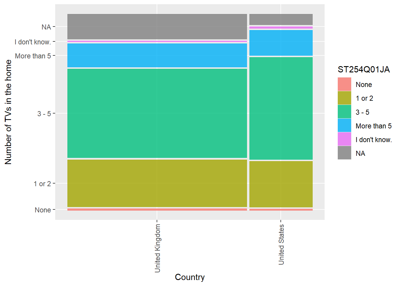

Show the code

# Rotate x-axis labels

In the UK, are there differences for boys and girls for the number of instruments in the home (ST251Q06JA)? Create a mosaic plot.

Show the code

# Create a data frame of instruments in the UK including gender

UKInstruments<-PISA_2022%>%
  select(CNT, ST251Q06JA, ST004D01T ) %>% 
  # choose CNT, no of instruments, gender
  filter(CNT == "United Kingdom") %>% # filter for the UK
  select(ST251Q06JA, ST004D01T) %>% 
  #drop the country variable now filtering is done
  droplevels() # Remove other countries which exist as factors


# Perform the test

kruskal.test(data = UKInstruments, ST251Q06JA ~ ST004D01T)


    Kruskal-Wallis rank sum test

data:  ST251Q06JA by ST004D01T
Kruskal-Wallis chi-squared = 15.366, df = 1, p-value = 8.859e-05

Show the code

# The p-value is less than 0.05 (p-value = 6.146e-07), therefore we reject the null hypothesis. Girls and boys have different access to instruments in the home.

# Create a geom_mosaic

ggplot(data = UKInstruments)+
  geom_mosaic(aes(x = product(ST251Q06JA, ST004D01T), fill = ST251Q06JA))+
  ylab("Number of instruments in the home for UK young people")+
  xlab("Gender")+
  theme(axis.text.x = element_text(angle = 90, vjust = 0.5, hjust=1))# Rotate x-axis labels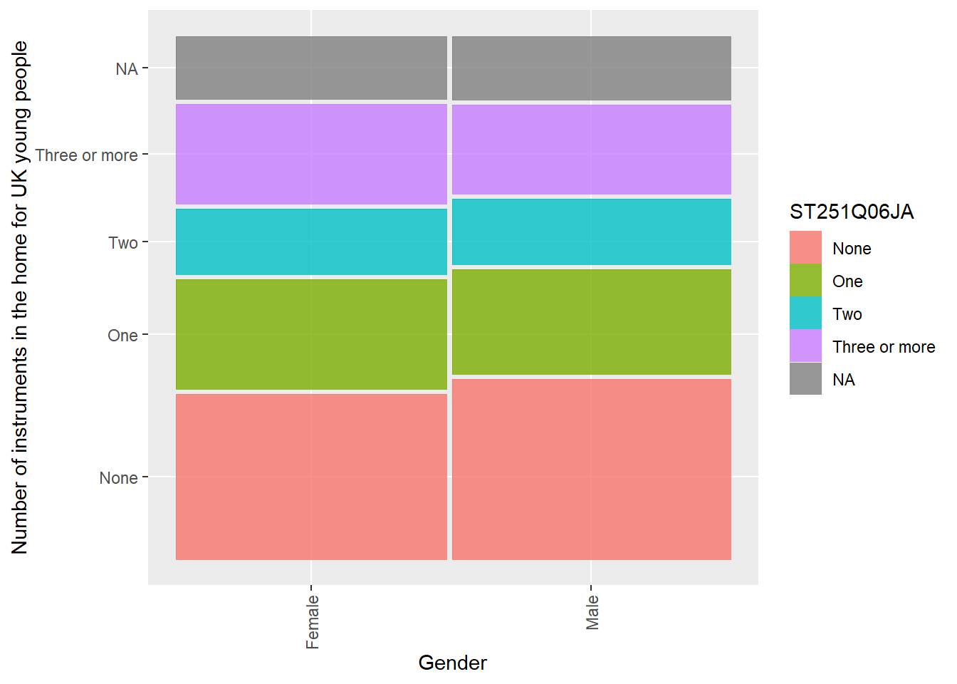

In the UK, are there differences for boys and girls working for pay in the UK (WORKPAY)? Plot the data as a mosaic plot.

Show the code

# Create a data frame of working in the Uk with gender

UKWork<-PISA_2022 %>%
  select(CNT, WORKPAY, ST004D01T) %>% # choose CNT, WORKPAY, gender
  filter(CNT == "United Kingdom") %>% # filter for the UK
  select(WORKPAY, ST004D01T)%>% 
  #drop the country variable now filtering is done
  droplevels() # Remove other countries which exist as factors

# Perform the test

kruskal.test(UKWork, WORKPAY ~ ST004D01T) # Perform the test


    Kruskal-Wallis rank sum test

data:  UKWork
Kruskal-Wallis chi-squared = 19522, df = 1, p-value < 2.2e-16

Show the code

# The p-value is less than 0.05 (p-value < 2.2e-16), therefore we reject the null hypothesis. Girls and boys have different levels of work

# Create a geom_mosaic

ggplot(data = UKWork)+
  geom_mosaic(aes(x = product(WORKPAY, ST004D01T), fill = WORKPAY))+
  ylab("Frequency of work")+
  xlab("Gender")+
  theme(axis.text.x = element_text(angle = 90, vjust = 0.5, hjust= 1))+
  theme(axis.text.y = element_text(size=rel(0.5))) # Reduce y-axis font size

Show the code

# Rotate x-axis labels

10 Extension tasks

Whilst chi-square tests are useful for reporting whether there are significant differences between the distribution of values in a contingency table, they don’t, by themselves tell you which cells in the contingency table differ from the expected values. To find out this information, you can do a post-hoc analysis. For example, imagine we are interested in if there are differences in the distribution of frequency of working for pay (WORKPAY ) in different countries. We create a subset of PISA data for the the UK, US, France and Germany (PISAsub), create a contingency table, plot the data, and perform the chisq.test.

PISAsub <- PISA_2022 %>%
  select(CNT, WORKPAY)%>% # choose country and type of school
  filter(CNT %in% c("United Kingdom", "United States", "France", "Germany"))%>% # filter by four countries
  droplevels() # Remove other countries which exist as factors

ContTab <- (xtabs(~CNT + WORKPAY, PISAsub)) # Create contingency table by CNT and school type

# Plot the data
ggplot(data = PISAsub)+
  geom_mosaic(aes(x = product(WORKPAY, CNT), fill = WORKPAY))+
  theme(axis.text.x = element_text(angle = 90, vjust = 0.5, hjust = 1))+
  theme(axis.text.y = element_text(size=rel(0.5))) # Reduce y-axis font size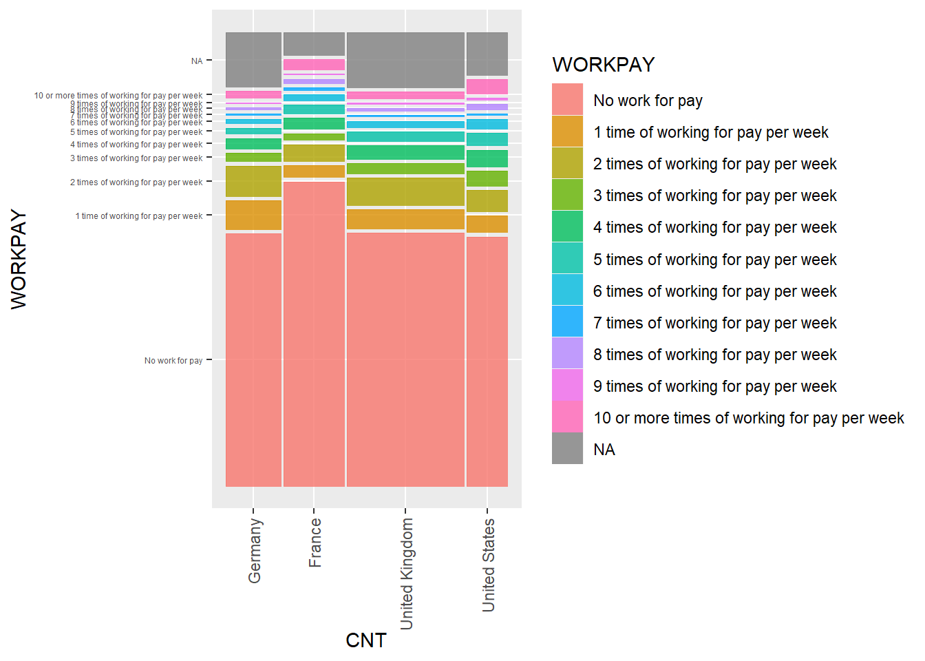

# perform the chi square test
chisq.test(ContTab)


    Pearson's Chi-squared test

data:  ContTab
X-squared = 534.25, df = 30, p-value < 2.2e-16

# perform the post hoc text
chisq.theo.multcomp(ContTab, p.method = "bonferroni")


        Pairwise comparisons using chi-squared tests

data:  ContTab and bonferroni

   observed.CNT                   observed.WORKPAY observed.Freq expected
        Germany                    No work for pay          3804    613.1
         France                    No work for pay          5074    613.1
 United Kingdom                    No work for pay          8079    613.1
  United States                    No work for pay          2794    613.1
        Germany 1 time of working for pay per week           431    613.1
      Chi  Pr(>Chi)    
 16994.58 0.000e+00 ***
 33214.42 0.000e+00 ***
 93034.38 0.000e+00 ***
  7938.89 0.000e+00 ***
    55.33 4.489e-12 ***
 [ reached 'max' / getOption("max.print") -- omitted 39 rows ]

P value adjustment method: bonferroni

In this case, the chi square test returns a p-value < 2.2e-16 suggesting significant differences between the countries. We can use the package RVAideMemoire to use the function chisq.theo.multcomp to perform the additional test.

The posthoc test returns a table of residuals and p-values for each cell in the contingency table The residuals give a sense how much each cell contributes to the total chi-squared value. The right most column (Pr(>Chi)) reports whether this deviation is statistically significant. All of the columns return a p-value below 0.05, as would be expected from the overall result, except for working for one time per week in the UK which has a p-value of 1.

10.1 Useful resources

11 Doing Chi-Square tests in R

You can find the code used in the video below

# Introduction to Chi-square
#
# Download data from /Users/k1765032/Library/CloudStorage/GoogleDrive-richardandrewbrock@gmail.com/.shortcut-targets-by-id/1c3CkaEBOICzepArDfjQUP34W2BYhFjM4/PISR/Data/PISA/subset/Students_2018_RBDP_none_levels.rds
# You want the file: Students_2018_RBDP_none_levels.rds
# and place in your own file system
# change loc to load the data directly. Loading into R might take a few minutes

loc <- "https://drive.google.com/open?id=14pL2Bz677Kk5_nn9BTmEuuUGY9S09bDb&authuser=richardandrewbrock%40gmail.com&usp=drive_fs"
PISA_2018 <- read_rds(loc)

# Are there differences between how often students change school?
# ST004D01T is the gender variable (Male, Female)
# SCCHANGE is a categorical variable (No change / One change / Two or more changes)

chidata <- PISA_2018 %>%
  select(CNT,ST004D01T,SCCHANGE) %>%
  filter(CNT=="United Kingdom")

chidata<-chidata[-c(1)]
chidata<-drop_na(chidata)

 chidata <- PISA_2018 %>%
   filter(CNT=="United Kingdom")
   select(ST004D01T,SCCHANGE) %>% 
   drop_na()
# Above is the approiach I took in the video
# An alternative, Pete suggests, which is more elegant, is below
# Note he drops the country varibale, within the piped section
# using: elect(-CNT)
#    
# chidata <- PISA_2018 %>%
#   select(CNT,ST004D01T,SCCHANGE) %>%
#   filter(CNT=="United Kingdom") %>%
#   select(-CNT) %>% 
#   drop_na()

# run the test
chisq.test(chidata$ST004D01T, chidata$SCCHANGE)

References

Baker, M. 2016. “Statisticians Issue Warning over Misuse of p Values.” Nature.

Cohen, Jacob. 1994. “The Earth Is Round (p<. 05).” American Psychologist 49 (12): 997.

Geher, Glenn, and Sara Hall. 2014. Straightforward Statistics: Understanding the Tools of Research. Oxford University Press, USA.