Self Study Tasks

The pages below set out a series of graded challenges that you can use to test your R and statistical skills. Sample code that solves each problem is included so you can compare your solution with ours. Don’t worry if you solve something in a different way, there will be multiple solutions to the same task. The tasks are all set on the PISA_2022 data set: PISA_2022

To load the data, use the code below:

0.1 Task 1 Practice creating a summary table #1

Create a table that summarises the mean PISA science scores by country. You will need to use the group_by, summarise and mean functions.

Show the code

PISAsummary<-PISA_2022%>%  # Pipe the overall frame to a summary data.frame
  select(CNT, PV1SCIE)%>%  # Select the two required columns
  group_by(CNT) %>%        # Group the entries by country
  summarise(meansci = mean(PV1SCIE)) # calculate means for each country

print(PISAsummary)

# A tibble: 80 × 2
   CNT                  meansci
   <fct>                  <dbl>
 1 Albania                 376.
 2 United Arab Emirates    436.
 3 Argentina               415.
 4 Australia               508.
 5 Austria                 494.
 6 Belgium                 495.
 7 Bulgaria                422.
 8 Brazil                  406.
 9 Brunei Darussalam       445.
10 Canada                  499.
# ℹ 70 more rows

Extension: use the signif function to give the responses to three significant figures

0.2 Task 2 Practice creating a summary table (including percentages) #2

Use the table function to create a summary of numbers of speakers of different languages (LANGN) recorded in the data frame for the UK. Use the mutate function to turn these into percentages (you will need to calculate a total)

Show the code

UKPISA<-PISA_2022%>%
  select(CNT,LANGN)%>%               # Select the country school type 
  filter(CNT == "United Kingdom")%>%  # filter for the UK
  select(LANGN) %>%                  # Just select the language (removing country)
  droplevels()                                   

UKPISA<-xtabs(data=UKPISA, ~ LANGN)  # Create a summary of counts
                                    # To manipulate the table it is
UKPISA<-as.data.frame(UKPISA)       # easier to convert it to a 
                                    # a data.frame

UKPISA<-mutate(UKPISA, per = Freq / sum(Freq)*100)
UKPISA  

                            LANGN Freq         per
1                           Scots  387  2.98334875
2                         English 9710 74.85353068
3                           Welsh  137  1.05612088
4                 Scottish Gaelic    7  0.05396238
5                           Irish   28  0.21584952
6  Other European languages (QSC)  154  1.18717237
7                    Ulster Scots   41  0.31606537
8   A non-European Union language  128  0.98674067
9          Another language (QUK)  809  6.23650940
10                        Missing 1571 12.11069997

Show the code

# If you want to sort the data (arrange descending by the percentage vector)
UKPISA<-UKPISA%>%
  arrange(desc(per))
UKPISA

                            LANGN Freq         per
1                         English 9710 74.85353068
2                         Missing 1571 12.11069997
3          Another language (QUK)  809  6.23650940
4                           Scots  387  2.98334875
5  Other European languages (QSC)  154  1.18717237
6                           Welsh  137  1.05612088
7   A non-European Union language  128  0.98674067
8                    Ulster Scots   41  0.31606537
9                           Irish   28  0.21584952
10                Scottish Gaelic    7  0.05396238

0.3 Task 3 Practice pivoting a table

Convert a table of UK Science, Maths and Reading scores, extracted from the main data set, into the long format R prefers. In the long format, each score becomes a single so each student will have three entries.

Show the code

# Create a data frame in wide format, with three columns for each student's scores (math, reading and science)
UKScores<-PISA_2022%>%
  select(CNT,PV1MATH, PV1READ, PV1SCIE)%>%
  filter(CNT == "United Kingdom")%>%
  select(PV1MATH, PV1READ, PV1SCIE)
# Use pivot longer to turn the three columns into one. First, pass pivotlonger the dataframe to be converted, then the three columns
# to convert into one, the name of the new longer column and the
# name of the new scores column

UKScores<-pivot_longer(UKScores, cols = c('PV1MATH', 'PV1READ', 'PV1SCIE'),
                       names_to = 'Subject', values_to = 'Score' )

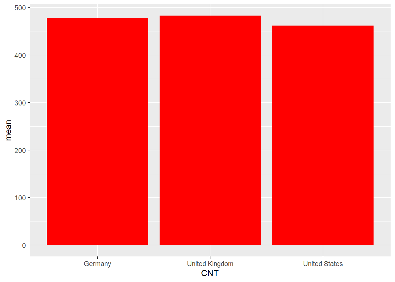
0.4 Task 4 Graphing Practice #1 A Bar Chart

Draw a bar chart of the mean mathematics scores for Germany, the UK, the US and China

Show the code

Plotdata<-PISA_2022%>%
  select(CNT, PV1MATH)%>%
  filter(CNT == "United Kingdom"| CNT == "United States"|
           CNT == "Germany"| CNT == "B-S-J-Z (China)")%>%
  group_by(CNT)%>%
  summarise(mean = mean(PV1MATH))

ggplot(Plotdata,               # Pass the data to be plotted to ggplot
       aes(x = CNT, y = mean))+    # set the x and y varibale
  geom_col(fill = "red")         # plot a column graph and fill in red

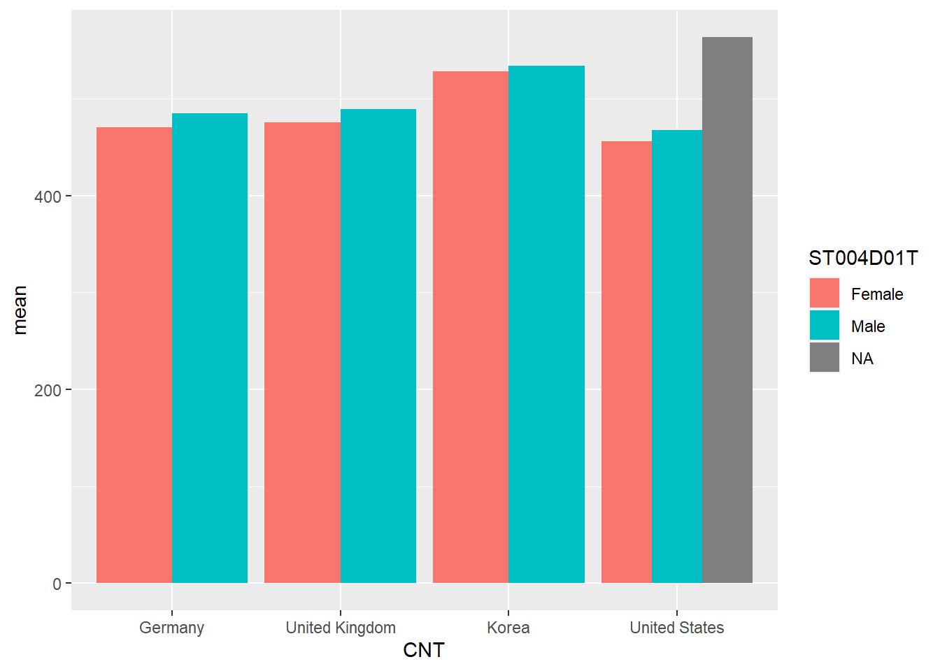
0.5 Task 5 Graphing Practice #2 A Bar Chart with two series

Draw a bar chart of the mean mathematics scores for Germany, the UK, the US and Korea for boys and girls

Show the code

Plotdata<-PISA_2022%>%
  select(CNT, PV1MATH, ST004D01T)%>%
  filter(CNT == "United Kingdom"|CNT=="United States"|
           CNT == "Germany"|CNT == "Korea")%>%
  group_by(CNT, ST004D01T)%>%
  summarise(mean = mean(PV1MATH))

ggplot(Plotdata,
       aes(x = CNT, y=mean, fill = ST004D01T))+ # Setting the fill to the gender
                                            # variable gives two series
  geom_col(position = position_dodge())     # position_dodge here means the

Show the code

                                            # means the bars are plotted                                                # side by side

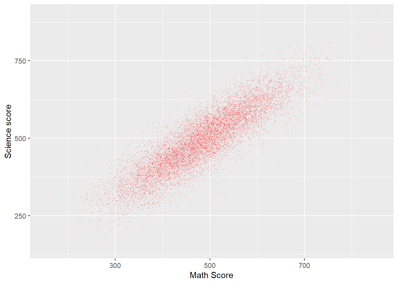
0.6 Task 6 Graphing Practice #3 A scatter plot

Plot a graph of science scores against mathematics scores for students in the UK

Show the code

Plotdata<-PISA_2022%>%              # Create a new data frame to be plotted
  select(CNT, PV1MATH, PV1SCIE)%>%  # Choose the country, and scores vectors
  filter(CNT == "United Kingdom")    # Filter for only Uk results

ggplot(Plotdata,                  # Pass the data to be plotted to ggplot
       aes(x = PV1MATH, y = PV1SCIE))+ # Define the x and y variable
      geom_point(size = 0.1, alpha = 0.2, colour="red")+ 
                                  # Use geom-point to create a scatter                                      # graph and set the size of the point 
                                    # alpha (i.e transparency)
      labs(x = "Math Score", y = "Science score") # Add clearer labels

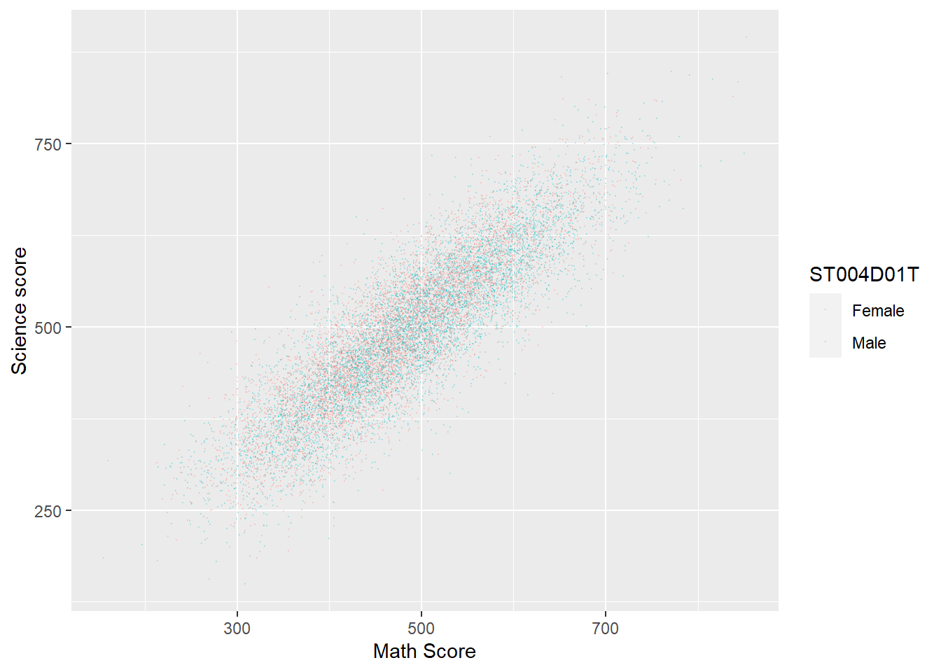
0.7 Task 7 Graphing Practice #4 A scatter plot with multiple series

Plot a graph of science scores against mathematics scores for students in the UK, with data split into two series for boys and girls

Show the code

Plotdata<-PISA_2022%>%              # Create a new dataframe to be plotted
  select(CNT, PV1MATH, PV1SCIE, ST004D01T)%>%  
  filter(CNT == "United Kingdom")    # Filter for only Uk results

ggplot(Plotdata,                  
       aes(x = PV1MATH, y = PV1SCIE, colour = ST004D01T))+ 
      geom_point(size = 0.1, alpha = 0.2)+ 
                          # As above, but set colour by the gender varibale
      labs(x = "Math Score", y = "Science score") 

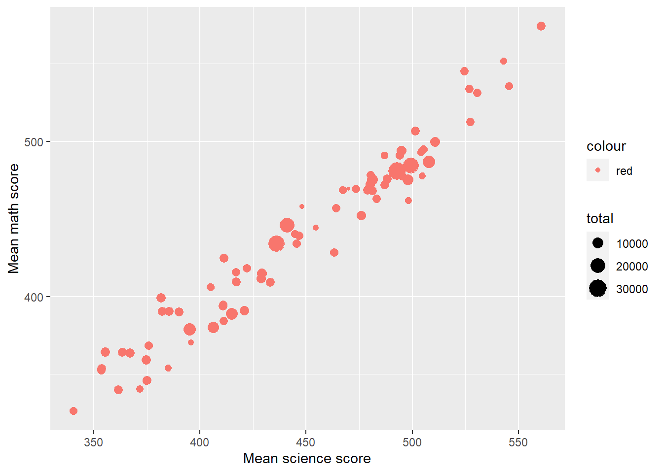
0.8 Task 8 Graphing Practice #4 A scatter plot with varying size points

Plot a graph of mean science scores against mean mathematics scores for all the countries in the data set. Vary the point size by the number of students per country.

Show the code

Plotdata<-PISA_2022%>%
  select(CNT, PV1MATH, PV1SCIE) %>%
  group_by(CNT) %>%
  summarise(meansci = mean(PV1SCIE), meanmath=mean(PV1MATH), total=n())

  # Summarise finds mean scores by countries and n() is used to sum
  # the number of students in each country

ggplot(Plotdata,
       aes(x = meansci, y = meanmath, size = total, colour = "red"))+
  # The size aesthetic is set to the total entries value computed
  # for the data set
  geom_point()+
  labs(x = "Mean science score", y = "Mean math score")

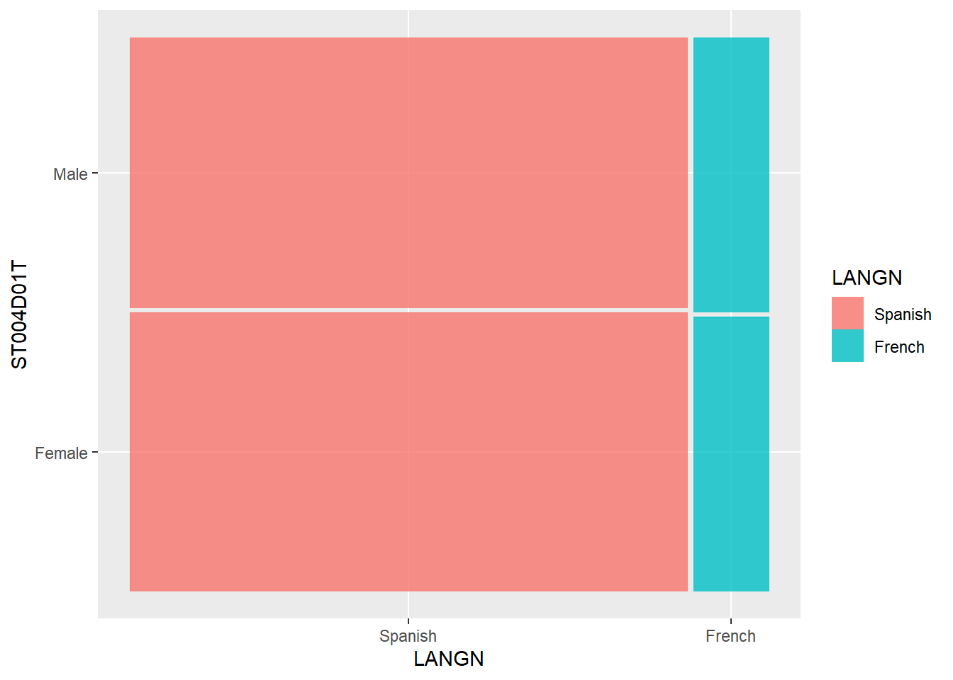
0.9 Task 9 Graphing Practice #5 A mosaic plot

Plot a mosaic plot of the number of students who speak (use LANGN) French and Spanish in the whole data set

Show the code

Lang<-PISA_2022 %>%
  select(ST004D01T, LANGN) %>%
  filter(LANGN == "French" | LANGN == "Spanish") %>%
  na.omit() %>%
  droplevels()

library(ggmosaic)
ggplot(Lang)+
  geom_mosaic(aes(x = product(ST004D01T, LANGN), fill = LANGN))

0.10 Task 10 T-test practice #1

Using the PISA 2022 data set, determine if there are statistically significant differences between the science, reading and mathematics scores of the UK and the US.

Show the code

# Create data frames with the score results for UK and US
UKscores<-PISA_2022%>%
  select(CNT,PV1MATH,PV1READ, PV1SCIE)%>%
  filter(CNT == "United Kingdom")

USscores<-PISA_2022%>%
  select(CNT,PV1MATH,PV1READ, PV1SCIE)%>%
  filter(CNT == "United States")

# Perform the t-test with maths results

t.test(UKscores$PV1MATH, USscores$PV1MATH)

    Welch Two Sample t-test

data:  UKscores$PV1MATH and USscores$PV1MATH
t = 12.614, df = 7958.4, p-value < 2.2e-16
alternative hypothesis: true difference in means is not equal to 0
95 percent confidence interval:
 17.45734 23.88158
sample estimates:
mean of x mean of y 
 482.5427  461.8733 

Show the code

# p-value is < 2.2e-16 so significant differences exist for maths

t.test(UKscores$PV1READ, USscores$PV1READ)

    Welch Two Sample t-test

data:  UKscores$PV1READ and USscores$PV1READ
t = -6.4317, df = 7555.2, p-value = 1.339e-10
alternative hypothesis: true difference in means is not equal to 0
95 percent confidence interval:
 -15.887576  -8.465219
sample estimates:
mean of x mean of y 
 490.7616  502.9380 

Show the code

# p-value = 1.339e-10 - statistically significant differences exist for reading between Uk and US

t.test(UKscores$PV1SCIE, USscores$PV1SCIE)

    Welch Two Sample t-test

data:  UKscores$PV1SCIE and USscores$PV1SCIE
t = -3.2425, df = 7545.7, p-value = 0.00119
alternative hypothesis: true difference in means is not equal to 0
95 percent confidence interval:
 -9.604044 -2.366899
sample estimates:
mean of x mean of y 
 492.2651  498.2506 

Show the code

# p-value = 0.00119  significant differences exist for science between the UK and US

0.11 Task 11 T-test practice #2

Divide the UK population into two groups, those that have internet access at home (ST250Q05JA) and those who do not. Are there statistically significant differences in the means of their reading, science and mathematics scores?

Show the code

# Create data frames with the score results for UK in two
# groups, has internet and no internet, based on ST011Q06TA

UKHasIntscores<-PISA_2022%>%
  select(CNT,PV1MATH,PV1READ, PV1SCIE, ST250Q05JA)%>%
  filter(CNT=="United Kingdom" & ST250Q05JA == "Yes")

UKNoIntscores<-PISA_2022%>%
  select(CNT,PV1MATH,PV1READ, PV1SCIE, ST250Q05JA)%>%
  filter(CNT=="United Kingdom" & ST250Q05JA == "No")

# Perform the t-test with maths results
t.test(UKHasIntscores$PV1MATH, UKNoIntscores$PV1MATH)

    Welch Two Sample t-test

data:  UKHasIntscores$PV1MATH and UKNoIntscores$PV1MATH
t = 10.177, df = 86.803, p-value < 2.2e-16
alternative hypothesis: true difference in means is not equal to 0
95 percent confidence interval:
  72.1637 107.1935
sample estimates:
mean of x mean of y 
 485.8926  396.2140 

Show the code

# p-value is < 2.2e-16 so no significant differences for maths scores from

# those with and without internet

t.test(UKHasIntscores$PV1READ, UKNoIntscores$PV1READ)

    Welch Two Sample t-test

data:  UKHasIntscores$PV1READ and UKNoIntscores$PV1READ
t = 10.117, df = 86.294, p-value = 2.547e-16
alternative hypothesis: true difference in means is not equal to 0
95 percent confidence interval:
  92.92909 138.37826
sample estimates:
mean of x mean of y 
 495.4067  379.7530 

Show the code

# p-value = 2.547e-16 so no signficant differences for reading scores from

# those with and without internet

t.test(UKHasIntscores$PV1SCIE, UKNoIntscores$PV1SCIE)

    Welch Two Sample t-test

data:  UKHasIntscores$PV1SCIE and UKNoIntscores$PV1SCIE
t = 9.3975, df = 86.657, p-value = 7.135e-15
alternative hypothesis: true difference in means is not equal to 0
95 percent confidence interval:
  73.60024 113.08755
sample estimates:
mean of x mean of y 
 495.8116  402.4677 

Show the code

# p-value = 7.135e-15 so no signficant differences for science scores from
# those with and without internet

0.12 Task 12 T-test practice #3

Using the PISA 2022 data set, are the mean mathematics scores of US boys and girls different to a statistically significant degree?

Show the code

# Create a data frame of US boys math scores

USboys <- PISA_2022 %>%
  select(CNT, PV1MATH, ST004D01T)%>%
  filter(CNT == "United States")

# Create a dataframe of US girls math scores

USgirls <- PISA_2022 %>%
  select(CNT, PV1MATH, ST004D01T) %>%
  filter(CNT == "United States")

# Perform the t-test, using $PVMATH to indicate which column of the data frame to use

t.test(USboys$PV1MATH, USgirls$PV1MATH)

    Welch Two Sample t-test

data:  USboys$PV1MATH and USgirls$PV1MATH
t = 0, df = 9102, p-value = 1
alternative hypothesis: true difference in means is not equal to 0
95 percent confidence interval:
 -3.90872  3.90872
sample estimates:
mean of x mean of y 
 461.8733  461.8733 

Show the code

# The p-value is 1 which is over 0.05 suggesting we accept the null hypothesis, there are no  statistically significant difference in US girls and boys math scores

0.13 Task 13 T-test practice #3

Are the mean science scores of all students in the US and the UK different to a statistically significant degree?

Show the code

# Create a data frame of US science scores

USSci<-PISA_2022 %>%
  select(CNT, PV1SCIE)%>%
  filter(CNT == "United States")

# Create a data frame of UK science scores

UKSci<-PISA_2022 %>%
  select(CNT, PV1SCIE)%>%
  filter(CNT == "United Kingdom")

# Perform the t-test, using $PV1SCIE to indicate which column of the dataframe to use

t.test(USSci$PV1SCIE, UKSci$PV1SCIE)

    Welch Two Sample t-test

data:  USSci$PV1SCIE and UKSci$PV1SCIE
t = 3.2425, df = 7545.7, p-value = 0.00119
alternative hypothesis: true difference in means is not equal to 0
95 percent confidence interval:
 2.366899 9.604044
sample estimates:
mean of x mean of y 
 498.2506  492.2651 

Show the code

# The p-value is 0.00119, less than 0.05, so we reject the null hypothesis, there are statistically significant differences between US and UK science scores  

0.14 Task 14 Kruskal Wallis practice #1

Are there statistically significant differences in the proportion of boys and girls who Working in household/take care of family members before or after school (WORKHOME) for the whole dataset? Note the responses are:

• No work in household or care of family members
• 1 time of working in household or caring for family members per week
• 2 times of working in household or caring for family members per week
• 3 times of working in household or caring for family members per week
• 4 times of working in household or caring for family members per week
• 5 times of working in household or caring for family members per week
• 6 times of working in household or caring for family members per week
• 7 times of working in household or caring for family members per week
• 8 times of working in household or caring for family members per week
• 9 times of working in household or caring for family members per week
• 10 or more times of working in household or caring for family members per week

Show the code

# Create a data frame of including gender and working or caring

workcare <- PISA_2022 %>%
  select(WORKHOME, ST004D01T) %>%
  filter(!is.na(WORKHOME))

# As the data are ordinal, use a kurskal wallis test

kruskal.test(data=workcare, WORKHOME ~ ST004D01T )

# p-value < 2.2e-16 so there are statistically significant differences between genders

# plot the results

workcare<-workcare %>%
  droplevels()%>%
  na.omit()

ggplot(data = workcare)+
   geom_mosaic(aes(x=product(WORKHOME, ST004D01T), fill=WORKHOME))+
  scale_y_discrete(label=abbreviate)

0.15 Task 15 Chi-square practice #1

Are there statistically significant differences, in the US, in the languages spoken (LANGN) by boys and girls?

Show the code

# Create a data frame of languages spoken in the US, including gender

USLang <- PISA_2022 %>%
  filter(CNT == "United States") %>%
  select(LANGN, ST004D01T) %>%
  na.omit() %>%
  droplevels()

# Create a contingency table

Contab <- xtabs(data=USLang, ~ LANGN + ST004D01T)

# Run the chi.sq test

chisq.test(Contab)

    Pearson's Chi-squared test

data:  Contab
X-squared = 7.9695, df = 3, p-value = 0.04665

Show the code

# The output p-value is 0.04665 which is less than 0.05. So reject the null hypothesis. There is a difference in language by gender

0.16 Task 16 Chi-square practice #3

Are there statistically significant differences in numbers of students missing school for more than 3 months because they were bored (ST261Q01JA) between the UK and US

Show the code

# ST261Q01JA - Why miss school for 3+ months: I was bored.
# Create a data frame for the two countries

Bored <- PISA_2022 %>%
  select(CNT, ST261Q01JA) %>%
  filter(CNT == "United Kingdom" | CNT == "United States") %>%
  droplevels() %>%
  na.omit()

# Create a contingency table

Contab <- xtabs(data=Bored, ~ CNT + ST261Q01JA)

# Do the chi squared test

chisq.test(Contab)

    Pearson's Chi-squared test with Yates' continuity correction

data:  Contab
X-squared = 26.573, df = 1, p-value = 2.537e-07

Show the code

# p-value is less than 0.05 (2.537e-07), so reject the null hypotheses - there are statistically significant differences in boredom in the UK and the US

0.17 Task 18 Anova practice #1

Are there statistically significant differences in mathematics scores of students in France, Germany, Spain, the UK and Italy? Find between which pairs of countries there are statistically significant differences in mathematics scores.

Show the code

# Create a data frame of the required countries

EuroPISA <- PISA_2022 %>%
  select(CNT, PV1MATH)%>%
  filter(CNT %in% c("Spain", "France", "United Kingdom", "Italy", "Germany"))

# Perform the anova

resaov <- aov(data = EuroPISA, PV1MATH ~ CNT)
summary(resaov)

               Df    Sum Sq Mean Sq F value Pr(>F)    
CNT             4   1236408  309102      39 <2e-16 ***
Residuals   67205 532663398    7926                   
---
Signif. codes:  0 '***' 0.001 '**' 0.01 '*' 0.05 '.' 0.1 ' ' 1

Show the code

# Yes, statistically significant differences exist between the countries Pr(>F) <2e-16 ***
# Perform a Tukey HSD test

TukeyHSD(resaov)

  Tukey multiple comparisons of means
    95% family-wise confidence level

Fit: aov(formula = PV1MATH ~ CNT, data = EuroPISA)

$CNT
                             diff         lwr       upr     p adj
Spain-Germany            3.140287  -0.2593483  6.539922 0.0862603
France-Germany          -9.679799 -13.9639526 -5.395645 0.0000000
United Kingdom-Germany   4.767983   1.0011433  8.534822 0.0050336
Italy-Germany           -2.548557  -6.4513428  1.354228 0.3845106
France-Spain           -12.820085 -16.0798407 -9.560330 0.0000000
United Kingdom-Spain     1.627696  -0.9141750  4.169566 0.4051954
Italy-Spain             -5.688844  -8.4281440 -2.949544 0.0000001
United Kingdom-France   14.447781  10.8066875 18.088875 0.0000000
Italy-France             7.131241   3.3496782 10.912805 0.0000027
Italy-United Kingdom    -7.316540 -10.5001420 -4.132937 0.0000000

Show the code

# Significant differences p<0.05 exist for all countries except: Spain-Germany; Italy-Germany, UK-Spain.

0.18 Task 19 Anova practice #2

For the UK PISA 2022 data set, which variable out of HOMEPOS, ST004D01T, OCOD1 (Mother’s occupation), OCOD2 (Father’s occupation), ST250Q05JA (having a link to the internet), and highest level of parental education (HISCED) accounts for the most variation in science score? What percentage of variance is explained by each variable?

! This is a big calculation so will take some time to compute !

Show the code

# Create a data frame for the UK
UKPISA_2022 <- PISA_2022 %>%
  filter(CNT == "United Kingdom")

# Perform the anova calculation with science score as the dependent variable

resaov <- aov(data=UKPISA_2022, 
              PV1SCIE ~ HOMEPOS + ST004D01T + OCOD1 + OCOD2 + ST250Q05JA + HISCED)

# Print the output
summary(resaov)

              Df   Sum Sq  Mean Sq  F value   Pr(>F)    
HOMEPOS        1 13423366 13423366 1571.542  < 2e-16 ***
ST004D01T      1   224779   224779   26.316 2.95e-07 ***
OCOD1        406  7197744    17728    2.076  < 2e-16 ***
OCOD2        483  6944691    14378    1.683  < 2e-16 ***
ST250Q05JA     1   110018   110018   12.880 0.000334 ***
HISCED         9  1636209   181801   21.284  < 2e-16 ***
 [ reached getOption("max.print") -- omitted 1 row ]
---
Signif. codes:  0 '***' 0.001 '**' 0.01 '*' 0.05 '.' 0.1 ' ' 1
2418 observations deleted due to missingness

Show the code

# Calculate the value of eta and multiple by a 100 to get the % of variance explained
eta <- etaSquared(resaov)
eta <- 100*eta
eta <- as.data.frame(eta)
eta

               eta.sq eta.sq.part
HOMEPOS    3.99268041   5.1441641
ST004D01T  0.32032198   0.4331991
OCOD1      4.63295284   5.9202525
OCOD2      6.12139253   7.6762624
ST250Q05JA 0.08516107   0.1155381
HISCED     1.46116663   1.9460370

Show the code

# The variable that explains most variation in science scores is father's occupation OCOD2 (7.7%), then home possession OCOD1 (5.9%), then wealth HOMEPOS (5.1%)