PISA

1 What is PISA

The Programme for International Student Assessment (PISA) is an OECD initiative that looks at the reading, mathematics and science abilities of students aged 15 years old. Data is collected from ~38 OECD countries and other partner countries every three years.

Dataset	Description	03	06	09	12	15	18	22
Student	demographic data on student participants	x	x	x	x	x	x	x
School	descriptive data about schools	x	x	x	x	x	x	x
Parent	a survey for student’s parents including information about home environments and parental education	x	x
Teacher	demographic, teaching, qualification and training data				x	x	x	x
Cognitive	individual results for each exam style question students took	x	x	x	x	x	x

PISA datasets above can be found on the OECD website. The links in the table above will allow you to download .parquet versions of these files which we have created, though they might need additional editing, e.g. reducing the number of columns or changing the types of each column. If you want to find out more about what each field stores, take a look at the corresponding codebook: 2022, 2018, 2015.

2 How to use it

The PISA datasets come in SPSS or SAS formats. The data used in this course comes directly from downloading the SPSS .sav files and using the haven package to clean it into a native R format suitable for analysis, in most cases .parquet files (see: ?@sec-parquet). There are a few quirks that you need to be aware of:

• R uses levels (factors) instead of labelled data
• All SPSS fields are labelled, and auto conversion into the native R data frame format would make numeric fields, factors(!?). To avoid this confusion we have stripped out the no-response data for numeric fields and replaced it with NA values. This means that you won’t be able to tell the reason that a field is missing, but most of the original data doesn’t appear to use the majority of these levels, i.e. there are few reasons given for missing data. The following labels have all been set to NA:

Labels set to NA in .parquet files

value	label
95	Valid Skip
97	Not Applicable
98	Invalid
99	No Response

• As the fields are now using R’s native factor format you might find that the data doesn’t quite match the format of the table labels. For example, CNT is labelled “Country code 3-character”, but the data is now instead the full country name.
• the examples shown in the book use cut down PISA data sets, where only a limited number of columns are included. The full datasets are linked in the table above.

2.1 Cleaning code

The .parquet files used in this book were produced using the following code.

First download the SPSS versions of the files from the OECD website, i.e. the .sav files.

Next create a function that converts .sav file columns to factors, picking up on a lot of edge cases:

# take an SPSS PISA dataframe and convert it to R factors

PISA_factorise <- function(df){
  # TODO: use SPSS types to make this more efficient
  # attr(df$x,"format.spss")
  
  # PISA data has almost everything labelled!
  # but not quite everything
  lbls <- map(df, function(x){
    attr(x, "label")
  })

  # label names for dud data
  dodgy_labels <- c(99995, 99997, 99998, 99999,
                    99999995, 99999997, 99999998, 99999999,
                    995, 997, 998, 999)
  dodgy <- c("Valid Skip", "Not Applicable", "Invalid", "No Response")
  dodgy2 <- c("N/A", "Invalid", "Missing")
  
  dfc <- df %>% # head(100) %>% #select(any_of(c("ST04Q01", "SCHOOLID", "TC002Q01NA"))) %>%
    mutate(across(everything(), 
                  function(x){
                    x_lbls <- attr(x, "labels")
                    x_lbl <- attr(x, "label")
                    
                    # outputs the current column name
                    message(cur_column())

                    # if it doesn't have labels to start with e.g. CNTSCHID
                    # do a direct copy
                    if(is.null(x_lbls)){
                      tmp <- x
                    }else if(cur_column() %in% c("ST03Q02", "ST03Q01") & 
                             "character" %in% class(x) &
                             grepl("Month", x_lbl)){
                      # for 2006/12 when date is a character?!
                        message("2006/12 - converting Month of birth character date to numeric")
                        tmp <- as.numeric(ifelse(grepl("^\\d+$", x), x, NA))
                        tmp[as.numeric(tmp) == 99] <- NA
                        tmp <- month.name[tmp]
                        tmp <- factor(tmp, levels=c(
                          "January", "February", "March", "April",
                          "May", "June", "July", "August",
                          "September", "October", "November", "December"
                        ))
                    }else if(cur_column() %in% c("ST03Q03", "ST03Q02") & 
                             "character" %in% class(x) &
                             grepl("Year", x_lbl)){
                      # for 2006/12 when date is a character?!
                      message("2006/12 - converting Year of birth character date to numeric")
                      tmp <- as.numeric(ifelse(grepl("^\\d+$", x), x, NA))
                      tmp[as.numeric(tmp) == 99] <- NA
                    }else if(cur_column() %in% c("CLCUSE301", "CLCUSE302", "Deffort") & 
                             "character" %in% class(x)){
                      # for 2012 when Effort-real  is a character?!
                      message("2012 - converting Effort-real/Deffort character to numeric")
                      tmp <- as.numeric(ifelse(grepl("^\\d+$", x), x, NA))
                      tmp[as.numeric(tmp) == 99] <- NA
                    }else if(cur_column() %in% c("VER_STU")){
                      # attr(,"format.spss")
                      # [1] "A7"
                      message("dealing with plain text from 2012 VERSTU")
                      tmp <- as.character(x)
                    }
                    else{
                      if(is.null(names(x)[1])){
                        first_name <- ""
                      }else{
                        first_name <- names(x)[1]
                      }
                      
                      if(first_name %in% c("SCHOOLID","StIDStd", "ST03Q01")){

                        #grepl("[a-zA-Z]", x[1]) # check to see if text contains character
                        
                        message(glue(">> {names(x)[1]} for 2012 so... character?"))
                        tmp <- x %>% as.character() %>% as.numeric()
                        
                        # filter out the dodgy NA values
                        tmp <- ifelse(as.numeric(tmp) %in% x_lbls,NA, tmp)
                        
                        # tmp <- x # can't convert to numeric?!
                        range(tmp, na.rm=TRUE)
                        
                      # if the labels are only for missing data set them to NA
                      }else if(setequal(names(x_lbls), dodgy)){
                        # replace any labelled data with NA
                       message(">> only missing labels, going numeric")
                       message(x[1:40])
                       tmp <- ifelse(as.numeric(x) %in% x_lbls,NA, x)
                        
                      # check that levels only contain 90s, if so likely numeric!
                      }else if(sum(as.numeric(x_lbls) >= 90 & 
                             as.numeric(x_lbls) < 100, na.rm=TRUE) == length(x_lbls)){
                        message(">> converting to numeric")
                        tmp <- ifelse(x >= 90,NA, x)
                      }else if(sum(as.numeric(x_lbls) %in% dodgy_labels) == length(x_lbls)){
                        message(">> weird LMINS etc")
                        tmp <- ifelse(x %in% dodgy_labels,NA, x)
                      }else{
                        message(">> normal factor")
                        tmp <- haven::as_factor(x)
                      }
                    }
                    # re attach label to each column
                    attr(tmp,"label") <- lbls[cur_column()][[1]]
                    message()
                    return(tmp)
                  }
    ))
 return(dfc) 
}

Finally, load the .sav file into R, run the conversion function, and save back to .parquet format:

# G:\My Drive\Kings\Code\PISR\code\

library(tidyverse)
library(glue)
library(openxlsx)
library(labelled)
library(haven)

base_folder <- "where/the/sav/files/are/stored/"

loc <- glue("{base_folder}pisa_student_2022.sav")
df <- read_spss(loc) # using haven

PISA_2022 <- PISA_factorise(df) # custom conversion code
write_parquet(PISA_2022, glue("{base_folder}pisa_student_2022.parquet"))

3 Common issues

The PISA datasets can be absolutely huge and might bring your computer to its knees; if you are using a computer with less than 16GB of RAM you might not be able to load some tables at all. Tables such as the Cognitive dataset have hundreds of thousands of rows and thousands of columns, loading them directly might lead to an error similar to this: Error: cannot allocate vector of size 2.1 Gb. This means that R can’t find enough RAM to load the dataset and has given up. You can see a rough estimate of how much RAM R is currently using the top Environment panel:

To get around this issues you can try to clean your current R environment using the brush tool:

This will drop all the current dataframes, objects, functions and packages that you have loaded meaning you will have to reload packages such as library(tidyverse) and library(haven) before you can attempt to reload the PISA tables.

A lack of RAM might also be the result of lots of other programs running concurrently on your computer. Try to close anything that you don’t need, web browsers can be particularly RAM hungry, so close them or as many tabs as you can.

If none of the above works, then please get in touch with the team, letting them know which table you need from which year, with which fields and for which countries. We will be able to provide you with a cutdown dataset.

4 Publishing your PISA analysis

So far you have been dealing with a subset of the data and the PV1 fields. Published analysis of PISA data, as with many other large scale data sets involves the weighted use of plausible values. In a nutshell the raw student sample from each country might not be a perfect representation of that country’s student population and the results of some students need to carry more weight than others to give you a proper picture of how that country is performing. Within a country, students won’t be able to complete every test element in the PISA question bank, so a range of plausible values are produced that predict how a students might have done if they had sat all the questions, based on their answers for the questions that they did sit. Due to these reasons, and others, you should always look at publications that refer to PISA with a certain degree of skepticism. A useful place to feed your skepticism is Jerrim’s 2020 video on Should the PISA findings be trusted?

“Almost nobody knows exactly where the OECD numbers come from” - Jerrim 2020

4.1 Plausible Values

In the PISA dataset, the outcomes of student tests are reported as plausible values, for example, in the variables of the science test (PV1SCIE, PV2SCIE, PV3SCIE, PV3SCIE, and PV5SCIE). It might seem counter intuitive that there are five or ten values for a score on a test. (note PISA published five plausible values before 2015, when they increased the number of plausible values to ten)

Plausible values (PVs) are a way of expressing the error in a measurement. The number of questions in the full PISA survey is very large, so students are randomly allocated to take a subset of questions (and even then, the test still takes two hours!). As no student completes the full set of questions - only 40% of students even answer questions in reading, science and mathematics (OECD 2014) - estimating how a student would have performed on the full question set involves some error. Plausible values are a way of expressing the uncertainty in the estimation of student scores.

One way of thinking of the PV scores is that they represent five or ten different estimates of students’ abilities based on the questions they have answered. To decrease measurement error, five different approaches are applied to create five different estimates, the PV scores.

The PISA Data Analysis Manual suggests:

Population statistics should be estimated using each plausible value separately. The reported population statistic is then the average of each plausible value statistic. For instance, if one is interested in the correlation coefficient between the social index and the reading performance in PISA, then five correlation coefficients should be computed and then averaged

Plausible values should never be averaged at the student level, i.e. by computing in the dataset the mean of the five plausible values at the student level and then computing the statistic of interest once using that average PV value. Doing so would be equivalent to an EAP estimate, with a bias as described in the previous section.

(Monseur et al. 2009, 100)

The actual PV values can differ substantially from each, for example if we work out the scaled (normalised) value for a PV value, that is how many standard deviations from the mean of other PV values a student gets we can see large fluctuations. For student 5, PV1SCIE is 0.147 standard deviations lower than the average of all students, but when we look at their PV2SCIE score, we see it is 1.10 standard deviations higher:

PISA_2022 %>% 
  mutate(PV1SCIE_z = scale(PV1SCIE),
         PV2SCIE_z = scale(PV2SCIE)) %>%
  select(PV1SCIE, PV2SCIE,
         PV1SCIE_z, PV2SCIE_z)

# A tibble: 613,744 × 4
    PV1SCIE PV2SCIE PV1SCIE_z[,1] PV2SCIE_z[,1]
      <dbl>   <dbl>         <dbl>         <dbl>
  1    335.    296.      -1.09         -1.47   
  2    315.    327.      -1.29         -1.17   
  3    359.    345.      -0.872        -1.00   
  4    215.    192.      -2.24         -2.45   
  5    435.    566.      -0.147         1.10   
  6    479.    482.       0.272         0.298  
  7    342.    290.      -1.03         -1.52   
  8    323.    359.      -1.22         -0.865  
  9    361.    362.      -0.854        -0.840  
 10    386.    427.      -0.614        -0.221  
 11    346.    322.      -0.990        -1.22   
 12    414.    432.      -0.346        -0.177  
 13    288.    332.      -1.55         -1.13   
 14    327.    362.      -1.18         -0.841  
 15    446.    459.      -0.0391        0.0835 
 16    340.    314.      -1.05         -1.29   
 17    394.    374.      -0.539        -0.725  
 18    569.    466.       1.13          0.153  
 19    386.    360.      -0.610        -0.863  
 20    369.    308.      -0.772        -1.35   
 21    468.    401.       0.170        -0.471  
 22    358.    273.      -0.882        -1.69   
 23    386.    369.      -0.615        -0.770  
 24    357.    410.      -0.884        -0.387  
 25    446.    435.      -0.0409       -0.147  
 26    298.    321.      -1.45         -1.23   
 27    412.    447.      -0.367        -0.0278 
 28    348.    365.      -0.975        -0.814  
 29    393.    430.      -0.541        -0.191  
 30    421.    395.      -0.282        -0.529  
 31    254.    214.      -1.87         -2.24   
 32    325.    321.      -1.19         -1.23   
 33    565.    546.       1.09          0.906  
 34    289.    267.      -1.54         -1.74   
 35    481.    476.       0.295         0.240  
 36    302.    333.      -1.42         -1.11   
 37    331.    319.      -1.13         -1.25   
 38    288.    257.      -1.54         -1.83   
 39    453.    391.       0.0237       -0.563  
 40    468.    611.       0.166         1.52   
 41    387.    387.      -0.604        -0.607  
 42    302.    311.      -1.41         -1.32   
 43    415.    507.      -0.335         0.539  
 44    288.    350.      -1.54         -0.956  
 45    227.    181.      -2.12         -2.56   
 46    452.    468.       0.0143        0.167  
 47    236.    176.      -2.04         -2.61   
 48    297.    330.      -1.45         -1.15   
 49    374.    321.      -0.729        -1.23   
 50    393.    358.      -0.549        -0.876  
 51    335.    356.      -1.10         -0.892  
 52    379.    359.      -0.678        -0.866  
 53    443.    483.      -0.0669        0.314  
 54    287.    266.      -1.55         -1.75   
 55    345.    267.      -1.000        -1.74   
 56    409.    417.      -0.391        -0.320  
 57    426.    359.      -0.235        -0.872  
 58    321.    286.      -1.23         -1.56   
 59    347.    329.      -0.981        -1.15   
 60    484.    468.       0.321         0.168  
 61    362.    293.      -0.844        -1.50   
 62    392.    382.      -0.559        -0.652  
 63    395.    424.      -0.524        -0.246  
 64    426.    445.      -0.237        -0.0474 
 65    328.    327.      -1.16         -1.17   
 66    398.    439.      -0.498        -0.104  
 67    315.    215.      -1.29         -2.24   
 68    540.    453.       0.854         0.0284 
 69    384.    408.      -0.629        -0.407  
 70    510.    464.       0.569         0.129  
 71    381.    367.      -0.663        -0.791  
 72    435.    375.      -0.145        -0.713  
 73    280.    294.      -1.62         -1.49   
 74    499.    489.       0.460         0.364  
 75    413.    450.      -0.359        -0.00711
 76    375.    285.      -0.714        -1.57   
 77    406.    385.      -0.419        -0.622  
 78    247.    231.      -1.94         -2.09   
 79    335.    366.      -1.10         -0.799  
 80    492.    438.       0.393        -0.115  
 81    463.    461.       0.121         0.103  
 82    324.    296.      -1.20         -1.47   
 83    264.    307.      -1.77         -1.36   
 84    288.    282.      -1.54         -1.60   
 85    308.    281.      -1.36         -1.61   
 86    303.    244.      -1.40         -1.96   
 87    274.    271.      -1.67         -1.71   
 88    311.    204.      -1.32         -2.34   
 89    401.    351.      -0.467        -0.944  
 90    338.    336.      -1.07         -1.08   
 91    376.    400.      -0.711        -0.475  
 92    330.    309.      -1.14         -1.34   
 93    354.    433.      -0.920        -0.166  
 94    358.    420.      -0.879        -0.290  
 95    304.    347.      -1.39         -0.981  
 96    362.    362.      -0.839        -0.840  
 97    355.    386.      -0.902        -0.612  
 98    396.    420.      -0.516        -0.288  
 99    376.    412.      -0.708        -0.368  
100    317.    266.      -1.27         -1.75   
101    275.    385.      -1.67         -0.622  
102    397.    394.      -0.509        -0.535  
103    347.    351.      -0.982        -0.948  
104    338.    398.      -1.07         -0.499  
105    229.    333.      -2.10         -1.12   
106    320.    349.      -1.24         -0.959  
107    490.    415.       0.375        -0.340  
108    422.    464.      -0.273         0.133  
109    357.    208.      -0.886        -2.31   
110    542.    556.       0.871         1.01   
111    273.    340.      -1.69         -1.05   
112    541.    496.       0.862         0.432  
113    305.    335.      -1.38         -1.10   
114    496.    476.       0.437         0.242  
115    260.    320.      -1.81         -1.24   
116    318.    317.      -1.26         -1.27   
117    327.    307.      -1.17         -1.36   
118    260.    273.      -1.81         -1.69   
119    315.    331.      -1.28         -1.13   
120    326.    300.      -1.18         -1.43   
121    402.    420.      -0.460        -0.286  
122    398.    425.      -0.500        -0.240  
123    216.    261.      -2.23         -1.80   
124    362.    321.      -0.839        -1.23   
125    361.    361.      -0.849        -0.846  
126    361.    312.      -0.853        -1.32   
127    423.    446.      -0.257        -0.0386 
128    320.    348.      -1.24         -0.971  
129    372.    448.      -0.745        -0.0212 
130    256.    182.      -1.85         -2.55   
131    456.    495.       0.0523        0.429  
132    345.    363.      -0.998        -0.826  
133    463.    497.       0.115         0.445  
134    408.    385.      -0.405        -0.623  
135    401.    447.      -0.465        -0.0340 
136    337.    364.      -1.08         -0.817  
137    320.    326.      -1.24         -1.18   
138    474.    458.       0.220         0.0719 
139    430.    465.      -0.197         0.142  
140    517.    515.       0.632         0.616  
141    317.    359.      -1.27         -0.869  
142    364.    360.      -0.826        -0.857  
143    490.    540.       0.378         0.852  
144    316.    311.      -1.28         -1.32   
145    307.    346.      -1.36         -0.994  
146    375.    424.      -0.722        -0.248  
147    328.    314.      -1.17         -1.30   
148    275.    290.      -1.66         -1.53   
149    249.    307.      -1.92         -1.37   
150    334.    314.      -1.11         -1.30   
151    258.    299.      -1.83         -1.44   
152    437.    420.      -0.126        -0.285  
153    312.    233.      -1.31         -2.06   
154    297.    332.      -1.45         -1.12   
155    426.    574.      -0.230         1.18   
156    476.    429.       0.243        -0.199  
157    339.    407.      -1.06         -0.408  
158    360.    449.      -0.860        -0.0116 
159    394.    357.      -0.534        -0.885  
160    428.    371.      -0.216        -0.753  
161    424.    409.      -0.253        -0.390  
162    347.    331.      -0.985        -1.14   
163    343.    370.      -1.02         -0.762  
164    286.    290.      -1.57         -1.52   
165    538.    532.       0.829         0.778  
166    327.    336.      -1.17         -1.09   
167    337.    350.      -1.08         -0.955  
168    347.    319.      -0.984        -1.25   
169    356.    269.      -0.893        -1.72   
170    368.    302.      -0.780        -1.41   
171    360.    395.      -0.861        -0.524  
172    457.    460.       0.0668        0.0958 
173    241.    288.      -1.99         -1.54   
174    359.    316.      -0.867        -1.28   
175    321.    316.      -1.23         -1.27   
176    245.    248.      -1.95         -1.92   
177    360.    317.      -0.862        -1.26   
178    391.    369.      -0.569        -0.776  
179    382.    276.      -0.654        -1.65   
180    291.    317.      -1.52         -1.27   
181    408.    405.      -0.401        -0.432  
182    274.    281.      -1.68         -1.61   
183    279.    281.      -1.63         -1.61   
184    292.    278.      -1.51         -1.64   
185    473.    446.       0.212        -0.0439 
186    380.    369.      -0.665        -0.772  
187    261.    298.      -1.80         -1.45   
188    464.    503.       0.127         0.499  
189    356.    351.      -0.898        -0.947  
190    340.    389.      -1.05         -0.580  
191    381.    293.      -0.663        -1.50   
192    472.    445.       0.201        -0.0537 
193    326.    313.      -1.19         -1.31   
194    318.    322.      -1.25         -1.22   
195    454.    454.       0.0382        0.0332 
196    287.    187.      -1.55         -2.50   
197    353.    360.      -0.929        -0.860  
198    511.    523.       0.575         0.692  
199    290.    296.      -1.52         -1.47   
200    564.    540.       1.08          0.856  
201    370.    391.      -0.766        -0.567  
202    456.    500.       0.0521        0.472  
203    251.    288.      -1.89         -1.54   
204    406.    385.      -0.421        -0.624  
205    238.    287.      -2.01         -1.55   
206    397.    384.      -0.503        -0.633  
207    426.    488.      -0.236         0.360  
208    422.    433.      -0.274        -0.169  
209    251.    379.      -1.90         -0.677  
210    542.    531.       0.871         0.767  
211    480.    448.       0.279        -0.0238 
212    268.    237.      -1.73         -2.03   
213    448.    446.      -0.0271       -0.0390 
214    317.    389.      -1.26         -0.581  
215    347.    249.      -0.984        -1.92   
216    360.    324.      -0.858        -1.20   
217    380.    383.      -0.667        -0.641  
218    274.    278.      -1.67         -1.64   
219    358.    361.      -0.874        -0.850  
220    358.    445.      -0.877        -0.0548 
221    270.    318.      -1.72         -1.26   
222    305.    264.      -1.38         -1.77   
223    369.    287.      -0.777        -1.55   
224    456.    532.       0.0524        0.781  
225    422.    432.      -0.275        -0.175  
226    282.    389.      -1.60         -0.580  
227    317.    375.      -1.26         -0.715  
228    363.    321.      -0.829        -1.23   
229    509.    492.       0.558         0.393  
230    377.    321.      -0.697        -1.23   
231    484.    507.       0.315         0.536  
232    379.    387.      -0.679        -0.603  
233    301.    310.      -1.42         -1.33   
234    405.    438.      -0.429        -0.115  
235    297.    276.      -1.46         -1.65   
236    436.    399.      -0.138        -0.484  
237    449.    460.      -0.0137        0.0918 
238    460.    567.       0.0912        1.11   
239    393.    343.      -0.544        -1.02   
240    587.    501.       1.30          0.477  
241    300.    275.      -1.43         -1.67   
242    460.    446.       0.0906       -0.0375 
243    402.    362.      -0.457        -0.842  
244    490.    494.       0.373         0.416  
245    389.    389.      -0.584        -0.582  
246    293.    276.      -1.49         -1.66   
247    434.    440.      -0.153        -0.102  
248    341.    400.      -1.04         -0.476  
249    323.    354.      -1.21         -0.916  
250    423.    438.      -0.261        -0.120  
251    320.    372.      -1.24         -0.748  
252    409.    391.      -0.395        -0.561  
253    522.    524.       0.684         0.702  
254    365.    346.      -0.812        -0.991  
255    496.    453.       0.436         0.0270 
256    468.    469.       0.162         0.174  
257    415.    441.      -0.338        -0.0866 
258    304.    414.      -1.39         -0.349  
259    273.    321.      -1.68         -1.23   
260    273.    264.      -1.68         -1.77   
261    344.    278.      -1.01         -1.64   
262    263.    314.      -1.78         -1.30   
263    310.    346.      -1.34         -0.991  
264    491.    437.       0.386        -0.126  
265    418.    396.      -0.306        -0.516  
266    523.    565.       0.685         1.09   
267    418.    406.      -0.306        -0.424  
268    312.    349.      -1.31         -0.962  
269    400.    300.      -0.478        -1.43   
270    330.    333.      -1.15         -1.12   
271    501.    435.       0.482        -0.148  
272    418.    436.      -0.312        -0.137  
273    425.    387.      -0.246        -0.598  
274    311.    318.      -1.32         -1.26   
275    469.    464.       0.178         0.129  
276    335.    283.      -1.10         -1.59   
277    575.    450.       1.18         -0.00740
278    368.    432.      -0.780        -0.170  
279    242.    281.      -1.98         -1.61   
280    515.    543.       0.615         0.876  
281    423.    310.      -0.262        -1.33   
282    344.    284.      -1.01         -1.58   
283    338.    327.      -1.06         -1.17   
284    305.    357.      -1.38         -0.889  
285    302.    310.      -1.41         -1.33   
286    411.    418.      -0.376        -0.307  
287    333.    343.      -1.11         -1.02   
288    262.    243.      -1.79         -1.97   
289    399.    366.      -0.485        -0.805  
290    338.    375.      -1.07         -0.712  
291    405.    356.      -0.433        -0.899  
292    428.    422.      -0.214        -0.273  
293    284.    277.      -1.58         -1.65   
294    341.    380.      -1.04         -0.664  
295    319.    371.      -1.25         -0.758  
296    401.    294.      -0.467        -1.49   
297    282.    317.      -1.60         -1.26   
298    381.    336.      -0.656        -1.09   
299    255.    268.      -1.86         -1.73   
300    467.    436.       0.162        -0.141  
301    367.    310.      -0.796        -1.34   
302    526.    546.       0.721         0.909  
303    325.    329.      -1.19         -1.16   
304    458.    430.       0.0747       -0.189  
305    312.    340.      -1.31         -1.04   
306    404.    401.      -0.443        -0.465  
307    412.    415.      -0.362        -0.338  
308    397.    340.      -0.507        -1.05   
309    420.    351.      -0.291        -0.941  
310    352.    459.      -0.937         0.0791 
311    577.    619.       1.20          1.61   
312    371.    384.      -0.757        -0.629  
313    290.    357.      -1.52         -0.885  
314    329.    226.      -1.16         -2.13   
315    435.    461.      -0.151         0.0994 
316    379.    367.      -0.679        -0.789  
317    572.    455.       1.16          0.0454 
318    487.    528.       0.350         0.743  
319    291.    336.      -1.52         -1.09   
320    266.    377.      -1.76         -0.693  
321    369.    379.      -0.769        -0.678  
322    314.    375.      -1.30         -0.713  
323    443.    349.      -0.0708       -0.963  
324    400.    414.      -0.478        -0.349  
325    404.    404.      -0.442        -0.441  
326    399.    366.      -0.487        -0.798  
327    367.    296.      -0.796        -1.47   
328    576.    634.       1.19          1.75   
329    288.    208.      -1.54         -2.30   
330    355.    313.      -0.904        -1.31   
331    467.    444.       0.159        -0.0615 
332    388.    326.      -0.591        -1.19   
333    231.    293.      -2.08         -1.50   
334    450.    442.      -0.00559      -0.0833 
335    490.    485.       0.377         0.328  
336    423.    424.      -0.263        -0.246  
337    217.    314.      -2.22         -1.30   
338    345.    353.      -1.00         -0.928  
339    464.    479.       0.130         0.275  
340    390.    342.      -0.579        -1.03   
341    439.    445.      -0.108        -0.0514 
342    289.    276.      -1.54         -1.65   
343    335.    302.      -1.09         -1.41   
344    236.    271.      -2.04         -1.70   
345    278.    445.      -1.64         -0.0533 
346    299.    414.      -1.44         -0.348  
347    324.    379.      -1.20         -0.679  
348    504.    491.       0.511         0.383  
349    270.    272.      -1.72         -1.69   
350    419.    462.      -0.297         0.112  
351    374.    417.      -0.729        -0.321  
352    224.    343.      -2.15         -1.02   
353    319.    345.      -1.25         -1.01   
354    401.    436.      -0.466        -0.137  
355    234.    196.      -2.05         -2.42   
356    401.    373.      -0.467        -0.733  
357    326.    345.      -1.19         -1.00   
358    430.    437.      -0.194        -0.127  
359    292.    245.      -1.51         -1.95   
360    436.    491.      -0.140         0.383  
361    489.    471.       0.363         0.196  
362    439.    391.      -0.105        -0.565  
363    345.    318.      -1.00         -1.26   
364    201.    310.      -2.37         -1.34   
365    521.    515.       0.666         0.612  
366    428.    493.      -0.214         0.408  
367    240.    268.      -2.00         -1.73   
368    231.    289.      -2.08         -1.53   
369    379.    310.      -0.683        -1.33   
370    378.    469.      -0.685         0.180  
371    410.    399.      -0.384        -0.491  
372    363.    354.      -0.826        -0.913  
373    194.    285.      -2.44         -1.57   
374    446.    322.      -0.0454       -1.22   
375    375.    360.      -0.714        -0.859  
376    275.    374.      -1.67         -0.725  
377    434.    391.      -0.158        -0.563  
378    281.    246.      -1.61         -1.94   
379    457.    503.       0.0629        0.503  
380    384.    360.      -0.631        -0.859  
381    311.    359.      -1.32         -0.864  
382    328.    311.      -1.17         -1.32   
383    318.    254.      -1.26         -1.86   
384    286.    270.      -1.56         -1.72   
385    311.    316.      -1.33         -1.27   
386    225.    355.      -2.14         -0.901  
387    292.    248.      -1.50         -1.92   
388    391.    359.      -0.562        -0.871  
389    470.    571.       0.182         1.15   
390    229.    303.      -2.10         -1.40   
391    525.    505.       0.705         0.518  
392    308.    284.      -1.35         -1.58   
393    303.    313.      -1.41         -1.30   
394    280.    321.      -1.62         -1.23   
395    371.    357.      -0.756        -0.888  
396    341.    389.      -1.04         -0.582  
397    453.    463.       0.0203        0.121  
398    417.    390.      -0.319        -0.574  
399    324.    262.      -1.20         -1.79   
400    269.    205.      -1.73         -2.33   
401    379.    394.      -0.677        -0.537  
402    304.    358.      -1.39         -0.874  
403    457.    412.       0.0654       -0.365  
404    334.    371.      -1.10         -0.752  
405    279.    358.      -1.63         -0.881  
406    388.    351.      -0.595        -0.946  
407    355.    313.      -0.903        -1.30   
408    341.    353.      -1.04         -0.921  
409    310.    316.      -1.33         -1.28   
410    353.    376.      -0.927        -0.707  
411    299.    310.      -1.44         -1.33   
412    571.    461.       1.14          0.0984 
413    220.    290.      -2.19         -1.52   
414    330.    298.      -1.14         -1.44   
415    351.    325.      -0.942        -1.19   
416    339.    334.      -1.06         -1.10   
417    506.    479.       0.531         0.274  
418    412.    305.      -0.367        -1.38   
419    514.    487.       0.605         0.349  
420    328.    326.      -1.16         -1.18   
421    393.    331.      -0.548        -1.14   
422    374.    481.      -0.730         0.293  
423    313.    294.      -1.30         -1.49   
424    424.    442.      -0.248        -0.0760 
425    338.    380.      -1.07         -0.670  
426    366.    373.      -0.801        -0.736  
427    369.    337.      -0.773        -1.08   
428    296.    293.      -1.47         -1.49   
429    405.    399.      -0.432        -0.484  
430    394.    464.      -0.534         0.126  
431    291.    292.      -1.52         -1.50   
432    176.    119.      -2.61         -3.15   
433    477.    391.       0.254        -0.560  
434    330.    384.      -1.14         -0.627  
435    348.    316.      -0.973        -1.28   
436    372.    377.      -0.746        -0.694  
437    460.    454.       0.0915        0.0311 
438    273.    297.      -1.69         -1.46   
439    306.    203.      -1.37         -2.35   
440    378.    312.      -0.690        -1.32   
441    487.    492.       0.345         0.400  
442    301.    326.      -1.42         -1.18   
443    342.    419.      -1.03         -0.295  
444    348.    370.      -0.976        -0.765  
445    452.    437.       0.0163       -0.127  
446    373.    383.      -0.736        -0.644  
447    276.    303.      -1.66         -1.40   
448    438.    351.      -0.120        -0.945  
449    408.    305.      -0.403        -1.39   
450    436.    428.      -0.139        -0.213  
451    343.    318.      -1.02         -1.26   
452    315.    351.      -1.28         -0.941  
453    355.    397.      -0.911        -0.506  
454    343.    379.      -1.02         -0.679  
455    550.    481.       0.943         0.294  
456    341.    309.      -1.04         -1.35   
457    372.    431.      -0.746        -0.184  
458    375.    357.      -0.712        -0.885  
459    318.    304.      -1.26         -1.39   
460    303.    239.      -1.40         -2.01   
461    352.    325.      -0.940        -1.19   
462    516.    437.       0.625        -0.126  
463    425.    372.      -0.238        -0.749  
464    240.    381.      -2.00         -0.660  
465    317.    373.      -1.27         -0.736  
466    521.    490.       0.673         0.376  
467    253.    297.      -1.87         -1.46   
468    419.    489.      -0.300         0.367  
469    218.    229.      -2.21         -2.11   
470    263.    281.      -1.78         -1.61   
471    530.    516.       0.758         0.624  
472    379.    402.      -0.678        -0.461  
473    418.    443.      -0.304        -0.0689 
474    431.    391.      -0.185        -0.562  
475    420.    377.      -0.294        -0.701  
476    436.    534.      -0.134         0.793  
477    274.    324.      -1.68         -1.20   
478    328.    382.      -1.16         -0.650  
479    455.    402.       0.0388       -0.457  
480    340.    314.      -1.05         -1.29   
481    340.    347.      -1.05         -0.979  
482    359.    395.      -0.867        -0.526  
483    548.    464.       0.922         0.127  
484    397.    402.      -0.510        -0.456  
485    343.    423.      -1.02         -0.257  
486    269.    244.      -1.73         -1.96   
487    430.    503.      -0.196         0.505  
488    285.    328.      -1.57         -1.16   
489    288.    210.      -1.55         -2.28   
490    354.    329.      -0.915        -1.15   
491    320.    341.      -1.24         -1.03   
492    304.    275.      -1.39         -1.66   
493    259.    332.      -1.82         -1.12   
494    584.    526.       1.26          0.717  
495    499.    483.       0.462         0.313  
496    460.    402.       0.0881       -0.463  
497    370.    374.      -0.768        -0.722  
498    333.    355.      -1.11         -0.903  
499    434.    422.      -0.158        -0.269  
500    287.    321.      -1.55         -1.23   
# ℹ 613,244 more rows

These differences make analysis at an individual student level hard to justify, though overall population or sub population scores will be more reliable. One approach that we could take to resolve the issue with using a single PV values would be to to look at using the average (here, taken to be the mean) of several PV scores. To calculate the mean of ten PV values, do the following (it might take some time to complete this calculation!):

PISA_2022 %>% 
  rowwise() %>%
  mutate(PV_SCIE_m = mean(c_across(matches("PV[0-9]+SCIE"))),
         PV_MATH_m = mean(c_across(matches("PV[0-9]+MATH"))),
         PV_READ_m = mean(c_across(matches("PV[0-9]+READ")))) %>%
  ungroup() %>% # to get rid of the rowwise operator
  select(PV_SCIE_m, PV_MATH_m, PV_READ_m)

This isn’t a perfect solution, and below we will take you through using Plausible Values correctly.

4.2 What are weights

The PISA data set contains two weighting variables that allow you to look at student outcomes that represent a country population accurately, and to compare countries against each other. When running our analysis, if we want it to be representative of the population, and allow for comparisons between countries, we should really be looking at the weighted scores. Luckily this can be easily done in R.

4.2.1 Student weights

The student weight, W_FSTUWT, represents the probability of an individual student being selected within a given country. For example, if PISA only sampled students from England for the UK results, then taking the mean Maths scores from these students probably wouldn’t be a representative score for all students in the UK including those from Wales, Scotland and Northern Ireland. In pratice PISA tries to sample students from all over a country, but it’s unlikely that the likelihood of a student being sampled in each region will be equal, it might also be the case that other factors are skewed, e.g. students from cities are more likely to be sampled than those from the countryside, or more affluent schools are more likely to be sampled than impoverished ones. To try and provide an accurate representation of the responses for different types of students across a whole country, PISA uses weights to increase or decrease the impact of individual students on overall results.

In the UK, students in Scotland had a higher likelihood of being sampled than those in England. With 4,763 students sampled in England and 3,257 sampled in Scotland; as a proportion, the Scottish population is too large. The school population of England (~9.1 million) is much larger than Scotland (~790 thousand), so we need to use weighting to decrease the impact of each Scottish student on the overall UK results, otherwise they would be over represented:

PISA_2022 %>% 
  filter(CNT == "United Kingdom") %>%
  group_by(REGION) %>%
  summarise(n=n(),
            W_FSTUWT_mean = mean(W_FSTUWT)) %>%
  gt() %>%
  fmt_number(columns = "n", decimals = 0) %>%
  fmt_number(columns = "W_FSTUWT_mean", decimals = 2) %>%
  cols_align(columns = "REGION", align="left")

REGION	n	W_FSTUWT_mean
Great Britain: England	4,763	131.04
Great Britain: Northern Ireland	2,384	9.47
Great Britain: Wales	2,568	12.73
Great Britain: Scotland	3,257	15.91

The ratio of students in England to students in Scotland is roughly 9,100,100 : 790,000 or 910 : 79, i.e. for every 910 English students, there should be 79 Scottish students; i.e. for every Scottish student there should be 11.5 English students. Applying the PISA students weights for students from England and Scotland we get:

(4763 * 131.04) / (3257 * 15.91)

[1] 12.04471

This is close to 11.5 but not quite the same as the population ratio. The reason might be that there are other factors that influence the student weighting, including situations where certain school types are under represented and other types over represented, for example there being more urban schools in the sample than in the population, this would then require students in rural schools to be given a greater weighting than students in urban schools. Allocating weights can be a complex process.

PISA_2022 %>% 
  filter(CNT == "United Kingdom") %>%
  group_by(REGION, W_FSTUWT) %>%
  count() %>%
  ungroup() %>%
  mutate(weight_label = ifelse(W_FSTUWT > 400, "Heavyweight!", NA)) %>%
  ggplot() + 
  geom_point(aes(x=W_FSTUWT, y=n, colour = W_FSTUWT < 400)) +
  geom_text(aes(x=W_FSTUWT-35, y=n-2, label=weight_label)) +
  facet_wrap(REGION~.) +
  theme_bw() +
  theme(legend.position = "none")

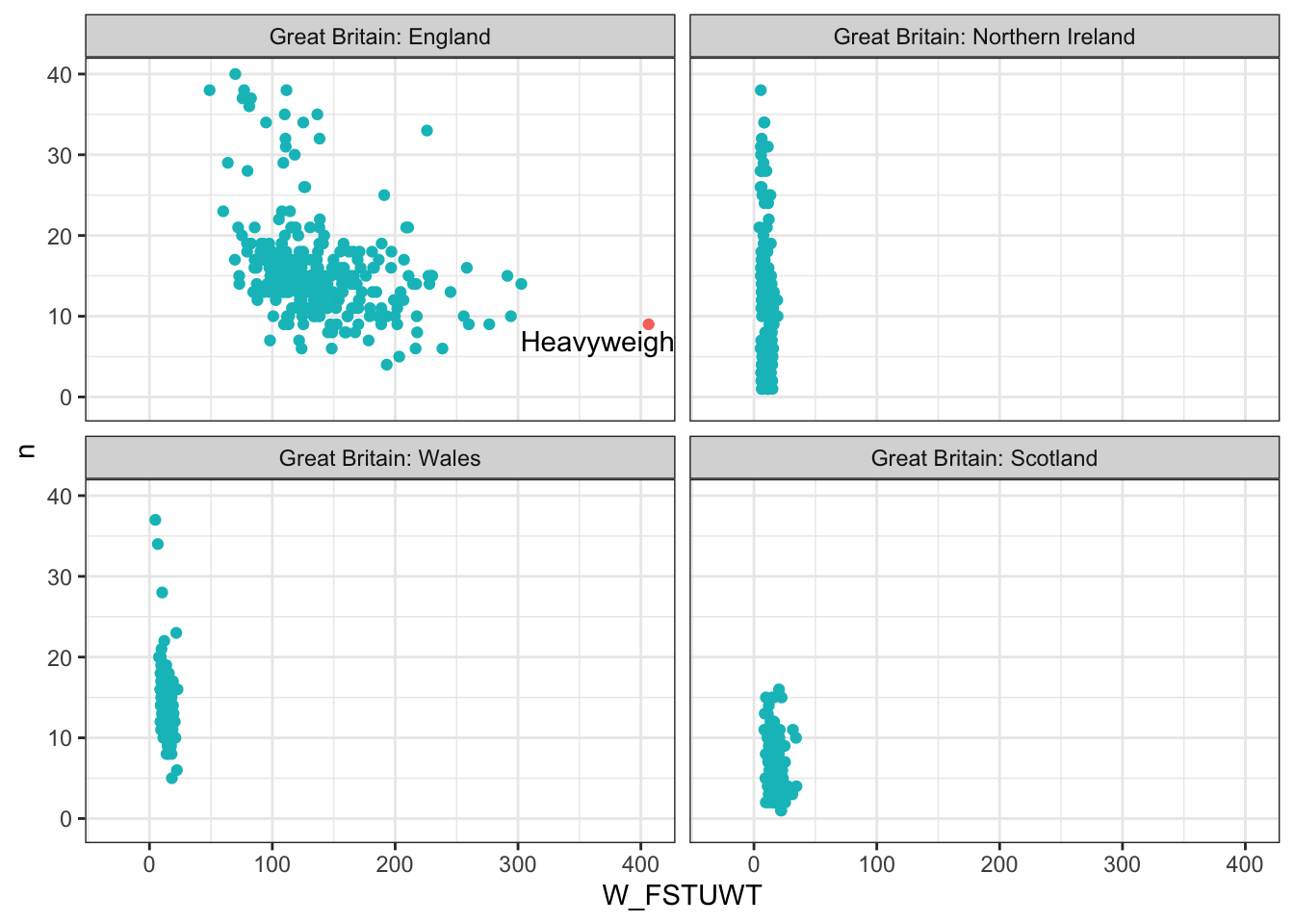
We can see that all students in England have a heavier weight attached to them than every student in Scotland, Wales and Northern Ireland. There is also a group of 9 students that have weightings of over 400, these are students that are very under represented in the sample. The weighting of these students is very high, and they will have a large impact on the overall results, potentially skewing results. For example, if the occupation of one of these student’s mothers (OCOD3) was as a butcher, then it would look like a lot of students in the UK had butchers as mothers, when in fact only one student in the sample did. This is a problem with weighting, and it is important to be aware of it when interpreting results.

So why are PISA sampling so many students from Scotland, Northern Ireland and Wales when each only forms a small part of the UK? By providing representative samples for each of these regions, it allows PISA to report for the UK as a whole and also to provide representative samples of students for each region of a country, allowing for the UK government (and us) to compare the performance of students under the different educational jurisdictions of the four nations.

So how do you use student weights in a calculation? Let’s look at some examples.

4.2.1.1 Numeric fields

We can find the mean poverty level of country, by looking at HOMEPOS. Calculating this without the weights gives us the following:

df <- PISA_2022 %>% 
  group_by(CNT) %>%
  summarise(HOMEPOS_m = mean(HOMEPOS, na.rm=TRUE),
            HOMEPOS_md = median(HOMEPOS, na.rm=TRUE)) %>%
  arrange(HOMEPOS_m)

df

# A tibble: 80 × 3
   CNT                          HOMEPOS_m HOMEPOS_md
   <fct>                            <dbl>      <dbl>
 1 Cambodia                      -2.41       -2.48  
 2 Morocco                       -1.77       -1.77  
 3 Philippines                   -1.75       -1.74  
 4 Indonesia                     -1.58       -1.63  
 5 El Salvador                   -1.57       -1.60  
 6 Guatemala                     -1.52       -1.58  
 7 Paraguay                      -1.52       -1.65  
 8 Palestinian Authority         -1.49       -1.43  
 9 Peru                          -1.40       -1.43  
10 Jordan                        -1.38       -1.36  
11 Panama                        -1.32       -1.31  
12 Mongolia                      -1.31       -1.36  
13 Dominican Republic            -1.31       -1.32  
14 Uzbekistan                    -1.30       -1.36  
15 Viet Nam                      -1.29       -1.30  
16 Colombia                      -1.26       -1.25  
17 Brazil                        -1.22       -1.30  
18 Thailand                      -1.17       -1.27  
19 Türkiye                       -1.08       -1.04  
20 Mexico                        -1.07       -1.12  
21 Baku (Azerbaijan)             -0.980      -1.02  
22 Costa Rica                    -0.979      -0.972 
23 Malaysia                      -0.908      -0.952 
24 Kazakhstan                    -0.870      -0.867 
25 Albania                       -0.859      -0.873 
26 Republic of Moldova           -0.846      -0.839 
27 Jamaica                       -0.834      -0.809 
28 Georgia                       -0.809      -0.817 
29 Argentina                     -0.806      -0.829 
30 Uruguay                       -0.747      -0.774 
31 Saudi Arabia                  -0.689      -0.767 
32 Kosovo                        -0.621      -0.633 
33 Ukrainian regions (18 of 27)  -0.550      -0.521 
34 North Macedonia               -0.490      -0.488 
35 Qatar                         -0.442      -0.477 
36 Romania                       -0.399      -0.357 
37 Chinese Taipei                -0.395      -0.407 
38 Chile                         -0.388      -0.396 
39 Bulgaria                      -0.368      -0.308 
40 Brunei Darussalam             -0.356      -0.411 
41 Montenegro                    -0.276      -0.269 
42 Greece                        -0.264      -0.268 
43 Macao (China)                 -0.253      -0.305 
44 Serbia                        -0.229      -0.201 
45 Japan                         -0.226      -0.210 
46 Hong Kong (China)             -0.198      -0.235 
47 Slovak Republic               -0.187      -0.125 
48 United Arab Emirates          -0.157      -0.208 
49 France                        -0.139      -0.0854
50 Croatia                       -0.117      -0.120 
51 Lithuania                     -0.0451     -0.0459
52 Latvia                         0.00480     0.0151
53 Israel                         0.0499      0.0954
54 Spain                          0.0739      0.104 
55 Portugal                       0.0755      0.0742
56 Poland                         0.0825      0.0847
57 Belgium                        0.0866      0.107 
58 Italy                          0.0887      0.109 
59 Hungary                        0.104       0.161 
60 United States                  0.115       0.0899
61 United Kingdom                 0.116       0.0947
62 Singapore                      0.124       0.0918
63 Germany                        0.149       0.188 
64 Finland                        0.162       0.217 
65 Estonia                        0.178       0.238 
66 Slovenia                       0.186       0.214 
67 Czech Republic                 0.194       0.239 
68 Switzerland                    0.221       0.260 
69 Denmark                        0.237       0.284 
70 Netherlands                    0.255       0.274 
71 Austria                        0.280       0.311 
72 Malta                          0.308       0.304 
73 Ireland                        0.318       0.319 
74 Sweden                         0.327       0.376 
75 Iceland                        0.346       0.383 
76 Canada                         0.348       0.366 
77 New Zealand                    0.367       0.401 
78 Korea                          0.371       0.418 
79 Australia                      0.483       0.520 
80 Norway                         0.547       0.616 

Now we can adjust this code to apply weights - students in each country will have their HOMEPOS score multiplied by their weight, the mean of these weighted HOMEPOS values calculated and the result of this divided by the mean weights for each country.

PISA_2022 %>% 
  group_by(CNT) %>%
  summarise(HOMEPOS_m_weight = 
              mean(HOMEPOS * W_FSTUWT, na.rm=TRUE) / 
              mean(W_FSTUWT)
            ) %>%
  arrange(HOMEPOS_m_weight) %>% 
  left_join(df) %>%
  mutate(weight_diff = abs((HOMEPOS_m - HOMEPOS_m_weight) / HOMEPOS_m))

# A tibble: 80 × 5
   CNT                         HOMEPOS_m_weight HOMEPOS_m HOMEPOS_md weight_diff
   <fct>                                  <dbl>     <dbl>      <dbl>       <dbl>
 1 Cambodia                            -2.34     -2.41       -2.48     0.0266   
 2 Philippines                         -1.75     -1.75       -1.74     0.000664 
 3 Morocco                             -1.74     -1.77       -1.77     0.0135   
 4 Indonesia                           -1.70     -1.58       -1.63     0.0738   
 5 El Salvador                         -1.63     -1.57       -1.60     0.0333   
 6 Paraguay                            -1.56     -1.52       -1.65     0.0259   
 7 Guatemala                           -1.54     -1.52       -1.58     0.00802  
 8 Palestinian Authority               -1.53     -1.49       -1.43     0.0270   
 9 Peru                                -1.44     -1.40       -1.43     0.0262   
10 Thailand                            -1.43     -1.17       -1.27     0.215    
11 Jordan                              -1.39     -1.38       -1.36     0.00733  
12 Colombia                            -1.37     -1.26       -1.25     0.0910   
13 Panama                              -1.32     -1.32       -1.31     0.00577  
14 Dominican Republic                  -1.31     -1.31       -1.32     0.00241  
15 Uzbekistan                          -1.31     -1.30       -1.36     0.00557  
16 Mongolia                            -1.31     -1.31       -1.36     0.00537  
17 Viet Nam                            -1.27     -1.29       -1.30     0.0128   
18 Brazil                              -1.23     -1.22       -1.30     0.0125   
19 Mexico                              -1.08     -1.07       -1.12     0.0102   
20 Türkiye                             -1.03     -1.08       -1.04     0.0437   
21 Baku (Azerbaijan)                   -1.02     -0.980      -1.02     0.0377   
22 Costa Rica                          -1.00     -0.979      -0.972    0.0242   
23 Kazakhstan                          -0.995    -0.870      -0.867    0.143    
24 Malaysia                            -0.925    -0.908      -0.952    0.0187   
25 Argentina                           -0.923    -0.806      -0.829    0.146    
26 Albania                             -0.866    -0.859      -0.873    0.00918  
27 Republic of Moldova                 -0.860    -0.846      -0.839    0.0165   
28 Georgia                             -0.832    -0.809      -0.817    0.0275   
29 Jamaica                             -0.786    -0.834      -0.809    0.0573   
30 Uruguay                             -0.768    -0.747      -0.774    0.0281   
31 Saudi Arabia                        -0.695    -0.689      -0.767    0.00840  
32 Kosovo                              -0.611    -0.621      -0.633    0.0169   
33 Chile                               -0.610    -0.388      -0.396    0.574    
34 Ukrainian regions (18 of 2…         -0.596    -0.550      -0.521    0.0854   
35 North Macedonia                     -0.500    -0.490      -0.488    0.0207   
36 Romania                             -0.478    -0.399      -0.357    0.199    
37 Qatar                               -0.470    -0.442      -0.477    0.0636   
38 Bulgaria                            -0.371    -0.368      -0.308    0.00632  
39 Brunei Darussalam                   -0.344    -0.356      -0.411    0.0329   
40 Chinese Taipei                      -0.332    -0.395      -0.407    0.161    
41 Greece                              -0.291    -0.264      -0.268    0.102    
42 Montenegro                          -0.283    -0.276      -0.269    0.0260   
43 Macao (China)                       -0.253    -0.253      -0.305    0.00187  
44 Slovak Republic                     -0.233    -0.187      -0.125    0.246    
45 Serbia                              -0.230    -0.229      -0.201    0.00396  
46 Japan                               -0.217    -0.226      -0.210    0.0393   
47 Hong Kong (China)                   -0.208    -0.198      -0.235    0.0522   
48 United Arab Emirates                -0.185    -0.157      -0.208    0.177    
49 Croatia                             -0.117    -0.117      -0.120    0.0000589
50 France                              -0.0718   -0.139      -0.0854   0.485    
51 Lithuania                           -0.0362   -0.0451     -0.0459   0.199    
52 Spain                                0.00557   0.0739      0.104    0.925    
53 Latvia                               0.00947   0.00480     0.0151   0.972    
54 Belgium                              0.0396    0.0866      0.107    0.543    
55 Portugal                             0.0499    0.0755      0.0742   0.339    
56 Hungary                              0.0502    0.104       0.161    0.518    
57 Poland                               0.0531    0.0825      0.0847   0.356    
58 Italy                                0.0738    0.0887      0.109    0.168    
59 Israel                               0.0757    0.0499      0.0954   0.517    
60 United Kingdom                       0.100     0.116       0.0947   0.135    
61 United States                        0.125     0.115       0.0899   0.0816   
62 Germany                              0.131     0.149       0.188    0.123    
63 Czech Republic                       0.132     0.194       0.239    0.321    
64 Singapore                            0.144     0.124       0.0918   0.166    
65 Estonia                              0.157     0.178       0.238    0.121    
66 Switzerland                          0.203     0.221       0.260    0.0802   
67 Slovenia                             0.231     0.186       0.214    0.239    
68 Austria                              0.248     0.280       0.311    0.112    
69 Finland                              0.260     0.162       0.217    0.602    
70 Netherlands                          0.265     0.255       0.274    0.0358   
71 Malta                                0.284     0.308       0.304    0.0798   
72 Ireland                              0.307     0.318       0.319    0.0345   
73 Sweden                               0.319     0.327       0.376    0.0227   
74 Iceland                              0.344     0.346       0.383    0.00730  
75 Korea                                0.357     0.371       0.418    0.0383   
76 New Zealand                          0.364     0.367       0.401    0.00932  
77 Denmark                              0.376     0.237       0.284    0.587    
78 Canada                               0.381     0.348       0.366    0.0933   
79 Australia                            0.478     0.483       0.520    0.0107   
80 Norway                               0.546     0.547       0.616    0.00202  

The mean values HOMEPOS_m are very close to the non weighted mean results, but note that some of the countries have now swapped places, with Thailand now making the bottom ten countries for this measure. In a world where people take international PISA rankings very seriously, weighting can make a big difference!

4.2.1.2 Categorical fields

If you want to work out the weighting of categorical fields you can do the following: (WARNING: check what to do with REGION)

# create a symbol of the focus_name
# allows you to adjust the focus of this code
# by changing the value in focus_name
focus_name <- "IC180Q01JA"
focus <- sym(focus_name)

df_weight <- PISA_2022 %>% 
  group_by(CNT, {{focus}}) %>%
  summarise(foc_weight = sum(W_FSTUWT)) %>%
  group_by(CNT, is.na({{focus}})) %>%
  mutate(foc_weight_pct = foc_weight / sum(foc_weight))

df_weight

# A tibble: 288 × 5
# Groups:   CNT, is.na(IC180Q01JA) [132]
    CNT                 IC180Q01JA foc_weight `is.na(IC180Q01JA)` foc_weight_pct
    <fct>               <fct>           <dbl> <lgl>                        <dbl>
  1 Albania             Strongly …     2507.  FALSE                       0.159 
  2 Albania             Disagree       5570.  FALSE                       0.354 
  3 Albania             Agree          5812.  FALSE                       0.369 
  4 Albania             Strongly …     1859.  FALSE                       0.118 
  5 Albania             <NA>          12678.  TRUE                        1     
  6 United Arab Emirat… <NA>          60765.  TRUE                        1     
  7 Argentina           Strongly …    45273.  FALSE                       0.145 
  8 Argentina           Disagree     117827.  FALSE                       0.377 
  9 Argentina           Agree        127605.  FALSE                       0.408 
 10 Argentina           Strongly …    21941.  FALSE                       0.0702
 11 Argentina           <NA>         283655.  TRUE                        1     
 12 Australia           Strongly …    10923.  FALSE                       0.0474
 13 Australia           Disagree      98093.  FALSE                       0.426 
 14 Australia           Agree        114875.  FALSE                       0.499 
 15 Australia           Strongly …     6476.  FALSE                       0.0281
 16 Australia           <NA>          34828.  TRUE                        1     
 17 Austria             Strongly …    10459.  FALSE                       0.163 
 18 Austria             Disagree      33042.  FALSE                       0.514 
 19 Austria             Agree         19061.  FALSE                       0.296 
 20 Austria             Strongly …     1778.  FALSE                       0.0276
 21 Austria             <NA>          11813.  TRUE                        1     
 22 Belgium             Strongly …    10347.  FALSE                       0.104 
 23 Belgium             Disagree      57077.  FALSE                       0.575 
 24 Belgium             Agree         29399.  FALSE                       0.296 
 25 Belgium             Strongly …     2515.  FALSE                       0.0253
 26 Belgium             <NA>          29303.  TRUE                        1     
 27 Bulgaria            Strongly …     6090.  FALSE                       0.177 
 28 Bulgaria            Disagree      14075.  FALSE                       0.409 
 29 Bulgaria            Agree         11369.  FALSE                       0.330 
 30 Bulgaria            Strongly …     2905.  FALSE                       0.0844
 31 Bulgaria            <NA>          18983.  TRUE                        1     
 32 Brazil              Strongly …   235724.  FALSE                       0.171 
 33 Brazil              Disagree     668596.  FALSE                       0.485 
 34 Brazil              Agree        387147.  FALSE                       0.281 
 35 Brazil              Strongly …    87035.  FALSE                       0.0631
 36 Brazil              <NA>         884469.  TRUE                        1     
 37 Brunei Darussalam   Strongly …      368.  FALSE                       0.0652
 38 Brunei Darussalam   Disagree       2919.  FALSE                       0.517 
 39 Brunei Darussalam   Agree          2203.  FALSE                       0.390 
 40 Brunei Darussalam   Strongly …      153.  FALSE                       0.0271
 41 Brunei Darussalam   <NA>            337.  TRUE                        1     
 42 Canada              <NA>         357911.  TRUE                        1     
 43 Switzerland         Strongly …     6965.  FALSE                       0.109 
 44 Switzerland         Disagree      32294.  FALSE                       0.507 
 45 Switzerland         Agree         22844.  FALSE                       0.358 
 46 Switzerland         Strongly …     1642.  FALSE                       0.0258
 47 Switzerland         <NA>          11951.  TRUE                        1     
 48 Chile               Strongly …    16894.  FALSE                       0.114 
 49 Chile               Disagree      68429.  FALSE                       0.463 
 50 Chile               Agree         54921.  FALSE                       0.371 
 51 Chile               Strongly …     7627.  FALSE                       0.0516
 52 Chile               <NA>          66238.  TRUE                        1     
 53 Colombia            <NA>         586683.  TRUE                        1     
 54 Costa Rica          Strongly …     7307.  FALSE                       0.157 
 55 Costa Rica          Disagree      24205.  FALSE                       0.519 
 56 Costa Rica          Agree         13593.  FALSE                       0.291 
 57 Costa Rica          Strongly …     1529.  FALSE                       0.0328
 58 Costa Rica          <NA>          10616.  TRUE                        1     
 59 Czech Republic      Strongly …     9050.  FALSE                       0.107 
 60 Czech Republic      Disagree      48233.  FALSE                       0.570 
 61 Czech Republic      Agree         24759.  FALSE                       0.293 
 62 Czech Republic      Strongly …     2576.  FALSE                       0.0304
 63 Czech Republic      <NA>          15648.  TRUE                        1     
 64 Germany             Strongly …    58565.  FALSE                       0.115 
 65 Germany             Disagree     260882.  FALSE                       0.514 
 66 Germany             Agree        176343.  FALSE                       0.348 
 67 Germany             Strongly …    11552.  FALSE                       0.0228
 68 Germany             <NA>         174057.  TRUE                        1     
 69 Denmark             Strongly …     1470.  FALSE                       0.0331
 70 Denmark             Disagree      14276.  FALSE                       0.321 
 71 Denmark             Agree         27339.  FALSE                       0.616 
 72 Denmark             Strongly …     1323.  FALSE                       0.0298
 73 Denmark             <NA>          12502.  TRUE                        1     
 74 Dominican Republic  Strongly …    17636.  FALSE                       0.220 
 75 Dominican Republic  Disagree      28924.  FALSE                       0.360 
 76 Dominican Republic  Agree         26915.  FALSE                       0.335 
 77 Dominican Republic  Strongly …     6825.  FALSE                       0.0850
 78 Dominican Republic  <NA>          41576.  TRUE                        1     
 79 Spain               Strongly …    45950.  FALSE                       0.116 
 80 Spain               Disagree     201512.  FALSE                       0.511 
 81 Spain               Agree        135443.  FALSE                       0.343 
 82 Spain               Strongly …    11756.  FALSE                       0.0298
 83 Spain               <NA>          64368.  TRUE                        1     
 84 Estonia             Strongly …      783.  FALSE                       0.0660
 85 Estonia             Disagree       5722.  FALSE                       0.482 
 86 Estonia             Agree          5098.  FALSE                       0.429 
 87 Estonia             Strongly …      269.  FALSE                       0.0226
 88 Estonia             <NA>           1473.  TRUE                        1     
 89 Finland             Strongly …     2297.  FALSE                       0.0481
 90 Finland             Disagree      20436.  FALSE                       0.428 
 91 Finland             Agree         23501.  FALSE                       0.492 
 92 Finland             Strongly …     1485.  FALSE                       0.0311
 93 Finland             <NA>          11236.  TRUE                        1     
 94 France              <NA>         781286.  TRUE                        1     
 95 United Kingdom      Strongly …    40671.  FALSE                       0.0811
 96 United Kingdom      Disagree     264813.  FALSE                       0.528 
 97 United Kingdom      Agree        186435.  FALSE                       0.372 
 98 United Kingdom      Strongly …     9545.  FALSE                       0.0190
 99 United Kingdom      <NA>         229760.  TRUE                        1     
100 Georgia             Strongly …     2740.  FALSE                       0.119 
101 Georgia             Disagree       7301.  FALSE                       0.318 
102 Georgia             Agree         10901.  FALSE                       0.475 
103 Georgia             Strongly …     2023.  FALSE                       0.0881
104 Georgia             <NA>          17450.  TRUE                        1     
105 Greece              Strongly …    18800.  FALSE                       0.223 
106 Greece              Disagree      49073.  FALSE                       0.582 
107 Greece              Agree         13515.  FALSE                       0.160 
108 Greece              Strongly …     2966.  FALSE                       0.0352
109 Greece              <NA>          13732.  TRUE                        1     
110 Guatemala           <NA>         168484.  TRUE                        1     
111 Hong Kong (China)   Strongly …     1740.  FALSE                       0.0397
112 Hong Kong (China)   Disagree      20067.  FALSE                       0.457 
113 Hong Kong (China)   Agree         20841.  FALSE                       0.475 
114 Hong Kong (China)   Strongly …     1221.  FALSE                       0.0278
115 Hong Kong (China)   <NA>           4376.  TRUE                        1     
116 Croatia             Strongly …     4086.  FALSE                       0.131 
117 Croatia             Disagree      17859.  FALSE                       0.573 
118 Croatia             Agree          8540.  FALSE                       0.274 
119 Croatia             Strongly …      680.  FALSE                       0.0218
120 Croatia             <NA>           3868.  TRUE                        1     
121 Hungary             Strongly …     7778.  FALSE                       0.102 
122 Hungary             Disagree      43124.  FALSE                       0.567 
123 Hungary             Agree         22753.  FALSE                       0.299 
124 Hungary             Strongly …     2363.  FALSE                       0.0311
125 Hungary             <NA>          11972.  TRUE                        1     
126 Indonesia           <NA>        3790846.  TRUE                        1     
127 Ireland             Strongly …     3283.  FALSE                       0.0546
128 Ireland             Disagree      34848.  FALSE                       0.580 
129 Ireland             Agree         21354.  FALSE                       0.355 
130 Ireland             Strongly …      630.  FALSE                       0.0105
131 Ireland             <NA>           5382.  TRUE                        1     
132 Iceland             Strongly …      216.  FALSE                       0.0650
133 Iceland             Disagree       1395.  FALSE                       0.420 
134 Iceland             Agree          1600.  FALSE                       0.482 
135 Iceland             Strongly …      108.  FALSE                       0.0324
136 Iceland             <NA>           1034.  TRUE                        1     
137 Israel              Strongly …    11806.  FALSE                       0.136 
138 Israel              Disagree      36260.  FALSE                       0.418 
139 Israel              Agree         35247.  FALSE                       0.406 
140 Israel              Strongly …     3519.  FALSE                       0.0405
141 Israel              <NA>          45644.  TRUE                        1     
142 Italy               Strongly …    52217.  FALSE                       0.119 
143 Italy               Disagree     246401.  FALSE                       0.561 
144 Italy               Agree        126434.  FALSE                       0.288 
145 Italy               Strongly …    13782.  FALSE                       0.0314
146 Italy               <NA>          57428.  TRUE                        1     
147 Jamaica             <NA>          25495.  TRUE                        1     
148 Jordan              Strongly …    23035.  FALSE                       0.246 
149 Jordan              Disagree      36245.  FALSE                       0.386 
150 Jordan              Agree         26399.  FALSE                       0.281 
151 Jordan              Strongly …     8106.  FALSE                       0.0864
152 Jordan              <NA>          50484.  TRUE                        1     
153 Japan               Strongly …   117347.  FALSE                       0.116 
154 Japan               Disagree     562095.  FALSE                       0.558 
155 Japan               Agree        305186.  FALSE                       0.303 
156 Japan               Strongly …    23135.  FALSE                       0.0230
157 Japan               <NA>          13606.  TRUE                        1     
158 Kazakhstan          Strongly …    24356.  FALSE                       0.0947
159 Kazakhstan          Disagree     110502.  FALSE                       0.430 
160 Kazakhstan          Agree        111368.  FALSE                       0.433 
161 Kazakhstan          Strongly …    10892.  FALSE                       0.0424
162 Kazakhstan          <NA>          15328.  TRUE                        1     
163 Cambodia            <NA>         126409.  TRUE                        1     
164 Korea               Strongly …    38662.  FALSE                       0.0961
165 Korea               Disagree     158940.  FALSE                       0.395 
166 Korea               Agree        194438.  FALSE                       0.483 
167 Korea               Strongly …    10124.  FALSE                       0.0252
168 Korea               <NA>          25848.  TRUE                        1     
169 Kosovo              <NA>          21045.  TRUE                        1     
170 Lithuania           Strongly …     2183.  FALSE                       0.101 
171 Lithuania           Disagree      11235.  FALSE                       0.519 
172 Lithuania           Agree          7687.  FALSE                       0.355 
173 Lithuania           Strongly …      527.  FALSE                       0.0244
174 Lithuania           <NA>           2618.  TRUE                        1     
175 Latvia              Strongly …     1010.  FALSE                       0.0674
176 Latvia              Disagree       7011.  FALSE                       0.468 
177 Latvia              Agree          6569.  FALSE                       0.438 
178 Latvia              Strongly …      394.  FALSE                       0.0263
179 Latvia              <NA>           1848.  TRUE                        1     
180 Macao (China)       Strongly …      187.  FALSE                       0.0428
181 Macao (China)       Disagree       2409.  FALSE                       0.552 
182 Macao (China)       Agree          1684.  FALSE                       0.386 
183 Macao (China)       Strongly …       81.7 FALSE                       0.0187
184 Macao (China)       <NA>             61.1 TRUE                        1     
185 Morocco             Strongly …    98434.  FALSE                       0.269 
186 Morocco             Disagree     153812.  FALSE                       0.420 
187 Morocco             Agree         98009.  FALSE                       0.268 
188 Morocco             Strongly …    15983.  FALSE                       0.0436
189 Morocco             <NA>          88748.  TRUE                        1     
190 Republic of Moldova <NA>          28879.  TRUE                        1     
191 Mexico              <NA>        1393727.  TRUE                        1     
192 North Macedonia     <NA>          16548.  TRUE                        1     
193 Malta               Strongly …      368.  FALSE                       0.118 
194 Malta               Disagree       1523.  FALSE                       0.489 
195 Malta               Agree          1095.  FALSE                       0.352 
196 Malta               Strongly …      128.  FALSE                       0.0409
197 Malta               <NA>            841.  TRUE                        1     
198 Montenegro          <NA>           6340.  TRUE                        1     
199 Mongolia            <NA>          40828.  TRUE                        1     
200 Malaysia            Strongly …    32108.  FALSE                       0.0894
201 Malaysia            Disagree     176408.  FALSE                       0.491 
202 Malaysia            Agree        138331.  FALSE                       0.385 
203 Malaysia            Strongly …    12108.  FALSE                       0.0337
204 Malaysia            <NA>          31493.  TRUE                        1     
205 Netherlands         <NA>         155987.  TRUE                        1     
206 Norway              <NA>          58970.  TRUE                        1     
207 New Zealand         <NA>          56382.  TRUE                        1     
208 Panama              Strongly …     5123.  FALSE                       0.194 
209 Panama              Disagree      10773.  FALSE                       0.407 
210 Panama              Agree          8530.  FALSE                       0.323 
211 Panama              Strongly …     2015.  FALSE                       0.0762
212 Panama              <NA>          15649.  TRUE                        1     
213 Peru                <NA>         499075.  TRUE                        1     
214 Philippines         <NA>        1782896.  TRUE                        1     
215 Poland              Strongly …    33869.  FALSE                       0.118 
216 Poland              Disagree     158147.  FALSE                       0.553 
217 Poland              Agree         83075.  FALSE                       0.291 
218 Poland              Strongly …    10811.  FALSE                       0.0378
219 Poland              <NA>          55659.  TRUE                        1     
220 Portugal            <NA>          96607.  TRUE                        1     
221 Paraguay            <NA>          81004.  TRUE                        1     
222 Palestinian Author… <NA>          88383.  TRUE                        1     
223 Qatar               <NA>          18348.  TRUE                        1     
224 Baku (Azerbaijan)   <NA>          30529.  TRUE                        1     
225 Ukrainian regions … Strongly …    13356.  FALSE                       0.108 
226 Ukrainian regions … Disagree      61379.  FALSE                       0.497 
227 Ukrainian regions … Agree         43666.  FALSE                       0.353 
228 Ukrainian regions … Strongly …     5137.  FALSE                       0.0416
229 Ukrainian regions … <NA>          42054.  TRUE                        1     
230 Romania             Strongly …    14905.  FALSE                       0.107 
231 Romania             Disagree      57042.  FALSE                       0.410 
232 Romania             Agree         59642.  FALSE                       0.428 
233 Romania             Strongly …     7665.  FALSE                       0.0550
234 Romania             <NA>          22765.  TRUE                        1     
235 Saudi Arabia        Strongly …    46886.  FALSE                       0.210 
236 Saudi Arabia        Disagree      87098.  FALSE                       0.389 
237 Saudi Arabia        Agree         70819.  FALSE                       0.316 
238 Saudi Arabia        Strongly …    18977.  FALSE                       0.0848
239 Saudi Arabia        <NA>          93671.  TRUE                        1     
240 Singapore           Strongly …     2342.  FALSE                       0.0575
241 Singapore           Disagree      19881.  FALSE                       0.488 
242 Singapore           Agree         17531.  FALSE                       0.430 
243 Singapore           Strongly …      970.  FALSE                       0.0238
244 Singapore           <NA>           1233.  TRUE                        1     
245 El Salvador         <NA>          68170.  TRUE                        1     
246 Serbia              <NA>          59250.  TRUE                        1     
247 Slovak Republic     Strongly …     5846.  FALSE                       0.148 
248 Slovak Republic     Disagree      19984.  FALSE                       0.507 
249 Slovak Republic     Agree         11868.  FALSE                       0.301 
250 Slovak Republic     Strongly …     1680.  FALSE                       0.0427
251 Slovak Republic     <NA>           8074.  TRUE                        1     
252 Slovenia            Strongly …     1788.  FALSE                       0.105 
253 Slovenia            Disagree       9389.  FALSE                       0.551 
254 Slovenia            Agree          5438.  FALSE                       0.319 
255 Slovenia            Strongly …      437.  FALSE                       0.0256
256 Slovenia            <NA>           1798.  TRUE                        1     
257 Sweden              Strongly …     6027.  FALSE                       0.0678
258 Sweden              Disagree      38935.  FALSE                       0.438 
259 Sweden              Agree         41143.  FALSE                       0.463 
260 Sweden              Strongly …     2797.  FALSE                       0.0315
261 Sweden              <NA>          19598.  TRUE                        1     
262 Chinese Taipei      Strongly …    15169.  FALSE                       0.0824
263 Chinese Taipei      Disagree     112090.  FALSE                       0.609 
264 Chinese Taipei      Agree         53582.  FALSE                       0.291 
265 Chinese Taipei      Strongly …     3232.  FALSE                       0.0176
266 Chinese Taipei      <NA>           6714.  TRUE                        1     
267 Thailand            Strongly …    47775.  FALSE                       0.0839
268 Thailand            Disagree     217575.  FALSE                       0.382 
269 Thailand            Agree        278841.  FALSE                       0.490 
270 Thailand            Strongly …    25345.  FALSE                       0.0445
271 Thailand            <NA>          35037.  TRUE                        1     
272 Türkiye             Strongly …   146806.  FALSE                       0.164 
273 Türkiye             Disagree     426210.  FALSE                       0.476 
274 Türkiye             Agree        283227.  FALSE                       0.316 
275 Türkiye             Strongly …    39236.  FALSE                       0.0438
276 Türkiye             <NA>          37923.  TRUE                        1     
277 Uruguay             Strongly …     2682.  FALSE                       0.114 
278 Uruguay             Disagree       9705.  FALSE                       0.411 
279 Uruguay             Agree         10061.  FALSE                       0.426 
280 Uruguay             Strongly …     1167.  FALSE                       0.0494
281 Uruguay             <NA>          17162.  TRUE                        1     
282 United States       Strongly …   192313.  FALSE                       0.0618
283 United States       Disagree    1515610.  FALSE                       0.487 
284 United States       Agree       1297432.  FALSE                       0.417 
285 United States       Strongly …   104544.  FALSE                       0.0336
286 United States       <NA>         551429.  TRUE                        1     
287 Uzbekistan          <NA>         482059.  TRUE                        1     
288 Viet Nam            <NA>         939459.  TRUE                        1     

4.2.1.3 T-tests

When performing t-tests, you can use the wtd.t.test() function from the weights package. This function allows you to perform a t-test with weights applied to the data. The wtd.t.test() function takes the following arguments:

library(weights)
wtd.t.test()

4.2.1.4 Correlations

If you’re looking to run a correlation test you’re going to need to adjust the number of observations depending on the weight of each student entry. For example if a student had a W_FSTUWT of 5, then you need to create 5 instances of that student, using the rep command, if another student had a weight of 105, you’d create 105 instances of that student; and so on. You then need to run the cor command on the enlarged data set. Note that we use the round command in the rep function as we need whole numbers for the weightings, this will lead to some potential, albeit very small, error in the final models.

cor_data <- PISA_2022 %>% 
  filter(CNT == "United Kingdom") %>%
  select(PV1MATH, ESCS, W_FSTUWT) %>%
  na.omit()

# create enlarged data set 
pv1math_weighted <- rep(cor_data$PV1MATH, 
                  times = round(cor_data$W_FSTUWT, 0))

escs_weighted <- rep(cor_data$ESCS, 
                  times = round(cor_data$W_FSTUWT, 0))

# run correlation test using weighted data
cor(pv1math_weighted, escs_weighted)

[1] 0.328924

If we run the correlation test on the original data set you can see that the correlation co-efficient is marginally different. Again, this might make the difference between something being statistically important or not.

cor(cor_data$PV1MATH, cor_data$ESCS)

[1] 0.3573955

If you do lots of correlations you could build your own function to perform this weighted test. Using the scale_weight parameter allows us to scale up the weighting value, so we can alleviate the issues of losing accuracy when rounding. For example if a weight for a student was 3.49 this would have been rounded down to 3, to fix this we could set scale_weight to 100, which would adjust the weight to 349 and would dissipate most of the rounding error.

corr_weighted <- function(data, fld1, fld2, 
                          fldweight = "W_FSTUWT", 
                          scale_weight = 1){
  cor_data <- data %>% 
    select(all_of(c(fld1, fld2, fldweight))) %>%
    na.omit()

  # create enlarged data set 
  fld1_weighted <- rep(cor_data[[fld1]], 
                    times = round(cor_data[[fldweight]] * scale_weight, 0))

  fld2_weighted <- rep(cor_data[[fld2]], 
                   times = round(cor_data[[fldweight]] * scale_weight, 0))

  # run correlation test using weighted data
  cor(fld1_weighted, fld2_weighted)
}


corr_weighted(data = PISA_2022, 
              fld1 = "PV1SCIE", 
              fld2 = "HOMEPOS",
              fldweight = "W_FSTUWT")

[1] 0.5189734

# we can just focus on females in France
corr_weighted(data = PISA_2022 %>% filter(CNT == "France", ST004D01T == "Female"), 
              fld1 = "PV1SCIE", 
              fld2 = "PV1MATH",
              fldweight = "W_FSTUWT")

[1] 0.8852219

# we can also omit the fldweight as the name is given
# by default in the function definition.
# by setting scale_weight to 100 we can get a slightly
# more accurate outcome
corr_weighted(data = PISA_2022 %>% filter(CNT == "France", ST004D01T == "Female"), 
              fld1 = "PV1SCIE", 
              fld2 = "PV1MATH",
              scale_weight = 100)

[1] 0.8852398

4.2.1.5 Linear models

When performing linear models, you can use the inbuilt weights argument in the lm() function. This is a simple way of applying weights to your model. The weights argument takes a vector of weights (in our case the column W_FSTUWT), which should be the same length as the number of rows in your data set.

lm(PV1MATH ~ PV1READ + ST004D01T,
   data = PISA_2022,
   weights = PISA_2022$W_FSTUWT) %>% 
  summary()

Call:
lm(formula = PV1MATH ~ PV1READ + ST004D01T, data = PISA_2022, 
    weights = PISA_2022$W_FSTUWT)

Weighted Residuals:
    Min      1Q  Median      3Q     Max 
-6291.5   -92.9    25.2   151.5  8580.0 

Coefficients:
               Estimate Std. Error t value Pr(>|t|)    
(Intercept)   8.561e+01  2.817e-01   303.9   <2e-16 ***
PV1READ       7.610e-01  6.021e-04  1263.8   <2e-16 ***
ST004D01TMale 2.161e+01  1.341e-01   161.2   <2e-16 ***
---
Signif. codes:  0 '***' 0.001 '**' 0.01 '*' 0.05 '.' 0.1 ' ' 1

Residual standard error: 354.7 on 613662 degrees of freedom
  (79 observations deleted due to missingness)
Multiple R-squared:  0.7227,    Adjusted R-squared:  0.7227 
F-statistic: 7.996e+05 on 2 and 613662 DF,  p-value: < 2.2e-16

lm(PV1MATH ~ PV1READ + ST004D01T,
   data = PISA_2022) %>% 
  summary()

Call:
lm(formula = PV1MATH ~ PV1READ + ST004D01T, data = PISA_2022)

Residuals:
     Min       1Q   Median       3Q      Max 
-289.474  -37.253   -2.099   35.295  309.126 

Coefficients:
               Estimate Std. Error t value Pr(>|t|)    
(Intercept)   8.363e+01  3.086e-01   271.0   <2e-16 ***
PV1READ       7.863e-01  6.478e-04  1213.8   <2e-16 ***
ST004D01TMale 2.528e+01  1.419e-01   178.2   <2e-16 ***
---
Signif. codes:  0 '***' 0.001 '**' 0.01 '*' 0.05 '.' 0.1 ' ' 1

Residual standard error: 55.2 on 613662 degrees of freedom
  (79 observations deleted due to missingness)
Multiple R-squared:  0.7062,    Adjusted R-squared:  0.7062 
F-statistic: 7.375e+05 on 2 and 613662 DF,  p-value: < 2.2e-16

If you are performing a linear regression on a subset of the data, you can use the filter() function to select the rows you want to include in your analysis. The weights argument will still work as long as the weights vector refers to the rows you have in your filtered data set. For example, if you want to run a linear regression on the UK data only, you can do the following:

lm(PV1MATH ~ PV1READ + ST004D01T,
   data = PISA_2022 %>% filter(CNT == "United Kingdom"),
   weights = PISA_2022 %>% filter(CNT == "United Kingdom") %>% pull(W_FSTUWT)) %>% 
  summary()

Call:
lm(formula = PV1MATH ~ PV1READ + ST004D01T, data = PISA_2022 %>% 
    filter(CNT == "United Kingdom"), weights = PISA_2022 %>% 
    filter(CNT == "United Kingdom") %>% pull(W_FSTUWT))

Weighted Residuals:
    Min      1Q  Median      3Q     Max 
-3198.7  -199.7   -16.5   164.9  2480.0 

Coefficients:
               Estimate Std. Error t value Pr(>|t|)    
(Intercept)   109.31499    2.42600   45.06   <2e-16 ***
PV1READ         0.73921    0.00462  160.02   <2e-16 ***
ST004D01TMale  28.26683    0.97996   28.84   <2e-16 ***
---
Signif. codes:  0 '***' 0.001 '**' 0.01 '*' 0.05 '.' 0.1 ' ' 1

Residual standard error: 417.6 on 12969 degrees of freedom
Multiple R-squared:  0.6661,    Adjusted R-squared:  0.666 
F-statistic: 1.293e+04 on 2 and 12969 DF,  p-value: < 2.2e-16

If we run the same model without the weights, we get a slightly different result.

lm(PV1MATH ~ PV1READ + ST004D01T,
   PISA_2022 %>% filter(CNT == "United Kingdom")) %>% 
  summary()

Call:
lm(formula = PV1MATH ~ PV1READ + ST004D01T, data = PISA_2022 %>% 
    filter(CNT == "United Kingdom"))

Residuals:
     Min       1Q   Median       3Q      Max 
-229.768  -36.901    0.317   36.857  243.155 

Coefficients:
               Estimate Std. Error t value Pr(>|t|)    
(Intercept)   1.083e+02  2.445e+00   44.27   <2e-16 ***
PV1READ       7.344e-01  4.685e-03  156.75   <2e-16 ***
ST004D01TMale 2.737e+01  9.829e-01   27.84   <2e-16 ***
---
Signif. codes:  0 '***' 0.001 '**' 0.01 '*' 0.05 '.' 0.1 ' ' 1

Residual standard error: 55.75 on 12969 degrees of freedom
Multiple R-squared:  0.6563,    Adjusted R-squared:  0.6563 
F-statistic: 1.238e+04 on 2 and 12969 DF,  p-value: < 2.2e-16

By default, above, the lm() function is treating all observations equally, regardless of their weights. Whilst the two models look very similar, a slight change in a p-value, or a change in the coefficient of a variable can have a big impact on the interpretation of a model.

4.2.2 Senate weights

The data set contains another weighting variable, the senate weight [COL_ID]. To ensure that countries make equal contributions to regression models when they have different response rates, senate weights are published (Jerrim et al. 2017). Senate weights renormalise the weights within each country so that the total for a country sums to a constant value, giving each country the same weight in an overall analysis (Rijmen 2011).

4.3 How do I use the plausible values and weights correctly?

To simplify our teaching, we focus on using a single PV value, PV1___ in our calculations. This is not the recommended use, but simplifies our introduction to the PISA data. Here we set out how to perform a more complete analysis.

The first step in analysis is to apply the weights. In the code below, we select the needed columns, country, the student weight column (W_FSTUWT) and the ten PV values (in this case for math). The mutate(across(... line multiples each of the ten PV values by the value in W_FSTUWT, the student weight, and adds new columns with _weighted appended.

PISA_2022 %>%
  select(CNT, W_FSTUWT, PV1MATH:PV10MATH) %>%
  mutate(across(PV1MATH:PV10MATH, ~ .x * W_FSTUWT, .names = "{.col}_weighted"))

Next we group_by(CNT) and summarise to get a total_weight for each country, by adding all the individual student weights (W_FSTUWT). To get a mean PV1, PV2, etc score for each country, we then sum all the weighted PV1 scores and divide by the total weight, and do the same for PV2, Pv3 etc. These are given the names PV1MATH_weighted_mean, PV2MATH_weighted_mean, etc.

PISA_2022 %>%
  select(CNT, W_FSTUWT, PV1MATH:PV10MATH) %>%
  mutate(across(PV1MATH:PV10MATH, ~ .x * W_FSTUWT, .names = "{.col}_weighted")) %>%
  group_by(CNT) %>%
  summarise(
    total_weight = sum(W_FSTUWT, na.rm = TRUE),
    across(PV1MATH_weighted:PV10MATH_weighted, ~ sum(.x, na.rm = TRUE) / total_weight, .names = "{.col}_mean"))

Finally, we calculated the mean of the PV1MATH_weighted_mean, PV2MATH_weighted_mean, … PV10MATH_weighted_mean columns. I have arranged the results in descending order.

PISA_2022 %>%
  select(CNT, W_FSTUWT, PV1MATH:PV10MATH) %>%
  mutate(across(PV1MATH:PV10MATH, ~ .x * W_FSTUWT, .names = "{.col}_weighted")) %>%
  group_by(CNT) %>%
  summarise(
    total_weight = sum(W_FSTUWT, na.rm = TRUE),
    across(PV1MATH_weighted:PV10MATH_weighted, ~ sum(.x, na.rm = TRUE) / total_weight, .names = "{.col}_mean")) %>%
  rowwise() %>%
  mutate(PV_mean_weighted = mean(c_across(ends_with("_mean")), na.rm = TRUE)) %>%
  select(CNT, PV_mean_weighted) %>%
  mutate(PV_mean_weighted = round(PV_mean_weighted, digits = 1)) %>%
  arrange(desc(PV_mean_weighted))

# A tibble: 80 × 2
# Rowwise: 
   CNT                          PV_mean_weighted
   <fct>                                   <dbl>
 1 Singapore                                575.
 2 Macao (China)                            552.
 3 Chinese Taipei                           547.
 4 Hong Kong (China)                        540.
 5 Japan                                    536.
 6 Korea                                    527.
 7 Estonia                                  510.
 8 Switzerland                              508 
 9 Canada                                   497.
10 Netherlands                              493.
11 Ireland                                  492.
12 Belgium                                  490.
13 Denmark                                  489.
14 United Kingdom                           489 
15 Poland                                   489 
16 Austria                                  487.
17 Australia                                487.
18 Czech Republic                           487 
19 Slovenia                                 484.
20 Finland                                  484.
21 Latvia                                   483.
22 Sweden                                   482.
23 New Zealand                              479.
24 Lithuania                                475.
25 Germany                                  475.
26 France                                   474.
27 Spain                                    473.
28 Hungary                                  473.
29 Portugal                                 472.
30 Italy                                    471.
31 Viet Nam                                 469.
32 Norway                                   468.
33 Malta                                    466 
34 United States                            465.
35 Slovak Republic                          464 
36 Croatia                                  463.
37 Iceland                                  459.
38 Israel                                   458.
39 Türkiye                                  453.
40 Brunei Darussalam                        442.
41 Ukrainian regions (18 of 27)             441.
42 Serbia                                   440.
43 United Arab Emirates                     431.
44 Greece                                   430.
45 Romania                                  428.
46 Kazakhstan                               425.
47 Mongolia                                 425.
48 Bulgaria                                 417.
49 Republic of Moldova                      414.
50 Qatar                                    414.
51 Chile                                    412.
52 Malaysia                                 409.
53 Uruguay                                  409.
54 Montenegro                               406.
55 Baku (Azerbaijan)                        397.
56 Mexico                                   395 
57 Thailand                                 394.
58 Peru                                     391.
59 Georgia                                  390 
60 Saudi Arabia                             389.
61 North Macedonia                          389.
62 Costa Rica                               385.
63 Colombia                                 383.
64 Brazil                                   379.
65 Argentina                                378.
66 Jamaica                                  377.
67 Albania                                  368.
68 Palestinian Authority                    366.
69 Indonesia                                366.
70 Morocco                                  365.
71 Uzbekistan                               364.
72 Jordan                                   361.
73 Panama                                   357.
74 Kosovo                                   355 
75 Philippines                              355.
76 Guatemala                                344.
77 El Salvador                              344.
78 Dominican Republic                       339.
79 Paraguay                                 338.
80 Cambodia                                 336.

This output matches the PISA published values for 2022.

Add @ http://repec.ioe.ac.uk/REPEc/pdf/qsswp1704.pdf

When performing tests (for example, t-tests or linear regressions) the recommended approach is to:Rubin’s rules for multiple imputation as recommended by the OECD OECD (2009a) : a) estimate a statistic multiple times, once each for each plausible value; b) average the values produced; c) estimate the magnitude of the imputation error; and d) calculate the final standard error from the sampling error and the imputation error.

Hence, if you were performing a linear model you should a) weight the raw scores you intend to use; b) run the model ten times, once each for each of the plausible values; c) calculate the average outcome metrics. For example, your code might look like this:

# a function that returns the models for a given formula
# formula must include exactly one PV
multi_pv_lm <- function(model_data,
                        pv_formula,
                        pv_vals = 1:10,
                        weight_id = "W_FSTUWT"){

  pv_focus_orig <- str_extract(pv_formula, "PV[0-9]+[A-Z]{4}")
  pv_focus <- pv_focus_orig %>% str_remove("PV[0-9]*")
  message("focusing on ", pv_focus)

  if(weight_id %in% names(model_data)){
    message(glue("Weighting by {weight_id}"))
  } else {
    message(glue("No {weight_id} weight variable found"))
    return(NULL)
  }
  
  # List of plausible value column names
  pv_columns <- paste0("PV", pv_vals, pv_focus)
  
  results <- map_dfr(pv_columns, \(pv){
    pv_formula_map <- str_replace(pv_formula, pv_focus_orig, pv)

    message(pv)
    # run model
    model <- lm(as.formula(pv_formula_map), 
                data = model_data, 
                weights = model_data[[weight_id]])
    # extract summary
    model_summary <- summary(model)
    
    # return rows
    broom::tidy(model_summary) %>% 
      mutate(R2 = model_summary$r.squared) %>%
      mutate(PV = pv)
  })
  
  results_flat <- results %>% 
    mutate(term = ifelse(str_detect(term, "PV[0-9]+[A-Z]{4}"), 
                         glue("PV_{pv_focus}"), 
                         term)) %>%
    group_by(term) %>% 
    summarise(estimate_mean = mean(estimate),
              estimate_sd = sd(estimate),
              std_error_mean = mean(std.error),
              std_error_sd = sd(std.error),
              statistic_mean = mean(statistic),
              statistic_sd = sd(statistic),
              p_value_mean = mean(p.value),
              p_value_sd = sd(p.value),
              r2 = max(R2))
  
  return(list(results=results, 
              results_flat=results_flat))
}

# we can call the model comparison, like so:
mdl_pvs_math <- multi_pv_lm(PISA_2022, "PV1MATH ~ HOMEPOS + ESCS")

# You can then access the full model responses through:
mdl_pvs_math$results

# A tibble: 30 × 7
   term        estimate std.error statistic p.value    R2 PV      
   <chr>          <dbl>     <dbl>     <dbl>   <dbl> <dbl> <chr>   
 1 (Intercept)    459.      0.131    3515.        0 0.290 PV1MATH 
 2 HOMEPOS         34.3     0.154     223.        0 0.290 PV1MATH 
 3 ESCS            10.7     0.153      69.8       0 0.290 PV1MATH 
 4 (Intercept)    459.      0.130    3524.        0 0.289 PV2MATH 
 5 HOMEPOS         34.4     0.154     224.        0 0.289 PV2MATH 
 6 ESCS            10.5     0.153      68.4       0 0.289 PV2MATH 
 7 (Intercept)    459.      0.130    3524.        0 0.290 PV3MATH 
 8 HOMEPOS         34.2     0.154     223.        0 0.290 PV3MATH 
 9 ESCS            10.8     0.153      70.6       0 0.290 PV3MATH 
10 (Intercept)    459.      0.130    3530.        0 0.291 PV4MATH 
11 HOMEPOS         34.4     0.153     224.        0 0.291 PV4MATH 
12 ESCS            10.6     0.152      69.3       0 0.291 PV4MATH 
13 (Intercept)    459.      0.130    3528.        0 0.292 PV5MATH 
14 HOMEPOS         34.5     0.154     224.        0 0.292 PV5MATH 
15 ESCS            10.7     0.153      70.1       0 0.292 PV5MATH 
16 (Intercept)    459.      0.131    3514.        0 0.290 PV6MATH 
17 HOMEPOS         34.3     0.154     223.        0 0.290 PV6MATH 
18 ESCS            10.7     0.153      70.0       0 0.290 PV6MATH 
19 (Intercept)    459.      0.130    3525.        0 0.291 PV7MATH 
20 HOMEPOS         34.5     0.154     225.        0 0.291 PV7MATH 
21 ESCS            10.5     0.153      68.9       0 0.291 PV7MATH 
22 (Intercept)    459.      0.130    3525.        0 0.292 PV8MATH 
23 HOMEPOS         34.4     0.154     224.        0 0.292 PV8MATH 
24 ESCS            10.8     0.153      70.6       0 0.292 PV8MATH 
25 (Intercept)    459.      0.130    3524.        0 0.291 PV9MATH 
26 HOMEPOS         34.3     0.154     223.        0 0.291 PV9MATH 
27 ESCS            10.7     0.153      70.1       0 0.291 PV9MATH 
28 (Intercept)    459.      0.130    3526.        0 0.292 PV10MATH
29 HOMEPOS         34.3     0.154     223.        0 0.292 PV10MATH
30 ESCS            10.9     0.153      71.6       0 0.292 PV10MATH

# or the mean values for model outcomes with:
mdl_pvs_math$results_flat

# A tibble: 3 × 10
  term      estimate_mean estimate_sd std_error_mean std_error_sd statistic_mean
  <chr>             <dbl>       <dbl>          <dbl>        <dbl>          <dbl>
1 (Interce…         459.       0.128           0.130     0.000189         3523. 
2 ESCS               10.7      0.140           0.153     0.000221           69.9
3 HOMEPOS            34.4      0.0896          0.154     0.000223          224. 
# ℹ 4 more variables: statistic_sd <dbl>, p_value_mean <dbl>, p_value_sd <dbl>,
#   r2 <dbl>

mdl_pvs_read <- multi_pv_lm(PISA_2022, "ESCS ~ HOMEPOS + PV1READ")

# TODO: https://bookdown.org/mwheymans/bookmi/rubins-rules.html

5 Questions

5.1 Where can I find examples of PISA test items?

The OECD do not release the full question set used in the PISA science, reading and mathematics tests in order to allow questions to be reused across cycles to allow valid inferences. However, you can find a document of items used in PISA 2000, 2003, 2006 and some test items here which give a flavour of the nature of the tests.

5.2 Why are some countries OECD countries and others aren’t?

The Organisation for Economic Co-operation and Development (OECD) has 38 member states. PISA is run by the OECD and its member states normally take part in each PISA cycle, but other countries are allowed to take part as Partners. You can find more details on participation here.

Results for OECD members are generally higher than for Partner countries:

PISA_2022 %>% 
  group_by(OECD) %>% 
  summarise(country_n = length(unique(CNT)),
            math_mean = mean(PV1MATH, na.rm=TRUE),
            math_sd = sd(PV1MATH, na.rm=TRUE),
            students_n = n())

# A tibble: 2 × 5
  OECD  country_n math_mean math_sd students_n
  <fct>     <int>     <dbl>   <dbl>      <int>
1 No           43      409.    97.8     318587
2 Yes          37      475.    95.0     295157

5.3 Why are the PV grades pivoting around the ~500 mark?

The scores for students in mathematics, reading and science are scaled so that the mean of students in OECD countries is roughly 500 points with a standard deviation of 100 points. To see this, run the following code:

PISA_2022 %>% 
  filter(OECD=="Yes") %>% 
  summarise(math_mean = mean(PV1MATH, na.rm=TRUE),
            math_sd = sd(PV1MATH, na.rm=TRUE),
            scie_mean = mean(PV1SCIE, na.rm=TRUE),
            scie_sd = sd(PV1SCIE, na.rm=TRUE),
            read_mean = mean(PV1READ, na.rm=TRUE),
            read_sd = sd(PV1READ, na.rm=TRUE))

# A tibble: 1 × 6
  math_mean math_sd scie_mean scie_sd read_mean read_sd
      <dbl>   <dbl>     <dbl>   <dbl>     <dbl>   <dbl>
1      475.    95.0      487.    101.      478.    104.

5.4 But the mean PV score isn’t 500?!

The OECD’s initial plan (in the 2000 study) was that the mean PC score for OECD countries should be 500 and the standard deviation 100 (OECD 2019a). However, after the 2000 study, scores were scaled to be comparable with the first cycle of data, resulting in means differing from 500 (Pulkkinen and Rautopuro 2022). For example, by 2015, the mean for science had fallen to 493 in science and reading, and 490 in mathematics.

5.5 Why are the letters TA and NA used in some field names?

5.6 How do I find fields that are numeric?

# using the following code!

nms <- PISA_2022 %>% select(where(is.numeric)) %>% names()
lbls <- map_dfr(nms,\(nme){
  message(nme)
  lbl <- attr(PISA_2022[[nme]], "label")
  row <- c(nme, lbl)
  names(row) <- c("name", "label")
  return(row)
})

5.7 How are schools and students selected to take part in PISA?

The students who take part in the PISA study are aged between 15 years and 3 (completed) months and 16 years and 2 (completed) months at the beginning of the testing period (OECD 2018). A number of classes of students can be excluded from data collection, up to 5% of all sampled students:

• Students classed as ‘functionally disabled’ so that they cannot participate in the test.
• Judged by teachers to have cognitive, emotional or behavioural difficulties that mean they cannot participate.
• The student lacks language abilities to take the test in the assessment language.
• There are no test material available in the student’s language
• Another agreed reason

The OECD expect that 85% of schools in their original sample participate - non participating schools can be replaced with a substitute, ‘replacement’ school. These replacement schools are similar in terms of a set of observable characteristics, that can be different depending on the country, for example in Canada this includes school funding and public/private school type. A minimum weighted response rate of 80% is required within schools.

The sampling strategy for PISA is a stratified two-stage sample design. That is schools are sampled to represent proportional distribution by size (referring to the number of enrolled 15-year-olds) sampling. Within schools, students are sampled with equal probability.

Schools are allowed to exclude students from their cohorts, based on the criteria given above. In 2015 the median exclusion rate from the sample was 3% for all OECD schools, with South Korea excluding 1% of students, and the UK excluding 8%.

(Jerrim2020?) argues that countries stretching the sampling rules above might allow for a country to lose 50% of eligible students from its sample and still be within the PISA rules for inclusion in the data set(!). In 2015, 91% of eligible student population in Japan were covered by the sampling, for the UK this was 69%, and for Canada, the top performing country for reading in that year’s study, the sample covered only 53% of the eligible student population.

Add Christian Bokhove papers https://bokhove.net/r-materials/

From the data, you can see that 50% of schools entered fewer than 30 students into PISA.

PISA_2022 %>% 
  group_by(CNTSCHID) %>%
  summarise(size = n()) %>%
  mutate(quartile = ntile(size, 4)) %>%
  group_by(quartile) %>%
  summarise(Qmax = max(size),
            Qmedian = median(size),
            Qmean = mean(size))

# A tibble: 4 × 4
  quartile  Qmax Qmedian Qmean
     <int> <int>   <dbl> <dbl>
1        1    19      10  10.1
2        2    30      25  25.2
3        3    37      34  33.8
4        4   475      40  44.4

ggplot(PISA_2022 %>% 
  group_by(CNTSCHID) %>%
  summarise(size = n()), aes(x=size)) +
  geom_density()

5.8 What are the PISA test questions like?

You can view sample PISA science, reading and mathematics questions here.

5.9 How can I find the ethnicity or race of a student taking the PISA test?

This data isn’t collected by PISA. Instead they collect information on the language spoken at home (LANGN) and the language of the test (LANGTEST_QQQ), as well as the immigration status and country of birth (COBN_S student, COBN_M mother, COBN_F father). Details on ethnicity and outcomes in the England are published through the country specific research report for 2018. Note that Chinese students are categorised under “Other” rather than “Asian” in UK data sets.

5.10 What are the PISA domains?

Every PISA test has included test items measuring literacy, numeracy and science. In each cycle, one of three areas is the focus of study (the major domain). In addition, extra domains have been added to cycles (for example, creative thinking and collaborative problem solving). The additional domains are shown in the table below.

Year	Major Domain	Minor Domains
2000	Reading literacy	Mathematics, Science
2003	Mathematics	Reading literacy, Science, Cross-curricular problem solving
2006	Science	Reading literacy, Mathematics
2009	Reading literacy	Mathematics, Science
2012	Mathematics	Reading literacy, Science, Creative problem solving
2015	Science	Mathematics, Reading literacy, Collaborative problem solving
2018	Reading literacy	Mathematics, Science, Global Competence
2022	Mathematics	Reading literacy, Science, Creative thinking
2025	Science	Mathematics, Reading literacy, Learning in the Digital World

5.11 Why is China given the CNT value B-S-J-Z (China) (2018) or B-S-J-G (China) (2015)?

B-S-J-G/Z (China) is an acronym for Beijing, Shanghai, Jiangsu and Guangdong/Zhejiang, the four provinces/municipalities of the People’s Republic of China that take part in PISA data collection. Zhejiang took the place of Guangdong in the 2018 dataset. Several authors (including (Du and Wong 2019)) comment that sampling only from some of the most developed regions of China means the country’s data is unlikely to be nationally representative.

5.12 Where is mainland China in PISA 2022?

Chinese provinces/municipalities (Beijing, Shanghai, Jiangsu and Zhejiang) and Lebanon are participants in PISA 2022 but were unable to collect data because schools were closed during the intended data collection period. - PISA 2022 participants

5.13 How do I calculate weighted means of the PV scores?

You can use a function written by Miguel Diaz Kusztrick, here is his slightly tidied function for calculating weighted means and standard deviations (original link):

# Copyright Miguel Diaz Kusztrick
wght_meansd_pv <- function(sdata, pv, weight, brr) {
    mmeans  <- c(0, 0, 0, 0)
    names(mmeans) <- c("MEAN","SE-MEAN","STDEV","SE-STDEV")
    
    mmeanspv <- rep(0,length(pv))
    stdspv   <- rep(0,length(pv))
    mmeansbr <- rep(0,length(pv))
    stdsbr   <- rep(0,length(pv))
    sum_weight <- sum(sdata[,weight])
    
    for (i in 1:length(pv)) {
        mmeanspv[i] <- sum(sdata[,weight]*sdata[,pv[i]])/sum_weight
        stdspv[i]   <- sqrt((sum(sdata[,weight]*(sdata[,pv[i]]^2))/swght)-mmeanspv[i]^2)
        for (j in 1:length(brr)) {
            sbrr<-sum(sdata[,brr[j]])
            mbrrj<-sum(sdata[,brr[j]]*sdata[,pv[i]])/sbrr
            mmeansbr[i]<-mmeansbr[i] + (mbrrj - mmeanspv[i])^2
            stdsbr[i]<-stdsbr[i] + (sqrt((sum(sdata[,brr[j]]*(sdata[,pv[i]]^2))/sbrr)-mbrrj^2) - stdspv[i])^2
        }       
    }
    mmeans[1] <- sum(mmeanspv) / length(pv)
    mmeans[2] <- sum((mmeansbr * 4) / length(brr)) / length(pv)
    mmeans[3] <- sum(stdspv) / length(pv)
    mmeans[4] <- sum((stdsbr * 4) / length(brr)) / length(pv)
    ivar <- c(0,0)
    
    for (i in 1:length(pv)) {
        ivar[1] <- ivar[1] + (mmeanspv[i] - mmeans[1])^2;
        ivar[2] <- ivar[2] + (stdspv[i] - mmeans[3])^2;
    }
    ivar = (1 + (1 / length(pv))) * (ivar / (length(pv) - 1));
    mmeans[2] <- sqrt(mmeans[2] + ivar[1]);
    mmeans[4] <- sqrt(mmeans[4] + ivar[2]);
    return(mmeans);
}

6 PISA quirks

6.1 Empty fields

GROSAGR Growth Mindset (WLE) seems to be completely missing for all countries:

All 2022 school responses to questions about the clubs and extra curricular activities run in a school SC053Q____ are coded as NA, as are SC207____. It’s not clear why this data is included in the dataset or whether this data should have values but doesn’t. These (albeit empty) fields are included in the full PISA_school_2022.parquet file linked above.

club_flds <- c("SC053Q01TA","SC053Q02TA","SC053Q03TA","SC053Q04TA","SC053Q05NA",
               "SC053Q06NA","SC053Q07TA","SC053Q08TA","SC053Q09TA","SC053Q10TA")

PISA_2022_school %>% 
  select(c("CNT", starts_with("SC053Q"), starts_with("SC207"))) %>% 
  group_by(CNT) %>%
  pivot_longer(-CNT, 
               names_to = "club",
               values_to = "present") %>%
  filter(!is.na(present)) %>%
  pull(club) %>% 
  unique()

# Note: SC053D11TA is present:
# <This academic year>,follow. activities/school offers<national modal grade for 15-year-olds>? <country specific item>

Additionally, creativity fields stored in ST334_____, ST340_____, ST341_____, PA185_____ and CREA____ on the student questionnaire are missing answers for all countries:

PISA_2022 <- read_feather(glue("{pisa_data}2022/PISA_student_2022.feather")) 
PISA_2022 %>% 
  select(c("CNT", 
           starts_with("ST334"),
           starts_with("ST340"), 
           starts_with("ST341"),
           starts_with("PA185"),
           starts_with("CREA"))) %>% 
  mutate(across(everything(), as.numeric)) %>%
  group_by(CNT) %>%
  pivot_longer(-CNT, 
               names_to = "creativity",
               values_to = "present") %>%
  filter(!is.na(present)) %>%
  pull(creativity) %>% 
  unique()

6.2 Cyprus present but missing

Cyprus is still present in the levels of CNT even though PISA hasn’t recorded data on Cyprus since 2012. Other countries that didn’t participate in the 2022 round have been removed from the levels, e.g. China.

countries <- PISA_2022 %>% pull(CNT) %>% unique()
country_lvls <- PISA_2022 %>% pull(CNT) %>% levels()
setdiff(country_lvls, countries)

6.3 Great Britain vs the United Kingdom

The United Kingdom is the country referred to when correctly combining the results of England, Scotland, Wales and Northern Ireland. However, the regions of the United Kingdom listed by the OECD are “Great Britain:” followed by England, Scotland, Wales and Northern Ireland. Northern Ireland isn’t part of Great Britain.

PISA_2022 %>% select(CNT, REGION) %>% 
  filter(grepl("Great Britain", REGION)) %>% distinct()

# A tibble: 4 × 2
  CNT            REGION                         
  <fct>          <fct>                          
1 United Kingdom Great Britain: Wales           
2 United Kingdom Great Britain: Northern Ireland
3 United Kingdom Great Britain: England         
4 United Kingdom Great Britain: Scotland        

6.4 How to spell “Ukrainian”

PISA records the language of the test sat by students in Ukraine LANGTEST_QQQ as “Ukranian” and the language they speak at home LANGN as “Ukrainian”

PISA_2022 %>%
  filter(CNT == "Ukrainian regions (18 of 27)") %>%
  group_by(LANGTEST_QQQ, LANGN) %>%
  count()

# A tibble: 11 × 3
# Groups:   LANGTEST_QQQ, LANGN [11]
   LANGTEST_QQQ LANGN                            n
   <fct>        <fct>                        <int>
 1 Russian      Russian                         16
 2 Russian      Ukrainian                        4
 3 Russian      Another language (UKR)           1
 4 Russian      Missing                          1
 5 Ukranian     Romani                           9
 6 Ukranian     Russian                        421
 7 Ukranian     Ukrainian                     3133
 8 Ukranian     Crimean Tatar Language (UKR)     9
 9 Ukranian     Another language (UKR)          56
10 Ukranian     Missing                        113
11 <NA>         Missing                        113

7 Interesting papers and reading on PISA

There are a number of useful OECD reports including:

• PISA Data Analysis Manual: SPSS second edition OECD (2009b);
• The PISA 2018 technical report OECD (2019b)
• PISA 2018 results OECD (2019a)
• PISA Adjusted 2021 design
• The PISA 2025 draft framework

John Jerrim and colleagues have written a number of papers which provide commentary on PISA analysis

• PISA 2012: how do results for the paper and computer tests compare? Jerrim (2016)
• To weight or not to weight?: The case of PISA data Jerrim et al. (2017)
• PISA 2015: how big is the ‘mode effect’ and what has been done about it? Jerrim et al. (2018)
• PISA 2018 in England, Northern Ireland, Scotland and Wales: Is the data really representative of all four corners of the UK? Jerrim (2021)
• Is Canada really an education superpower? The impact of non-participation on results from PISA 2015 Anders et al. (2021)
• Has Peak PISA passed? An investigation of interest in International Large-Scale Assessments across countries and over time Jerrim (2023)
• Conditioning: how background variables can influence PISA scores Zieger et al. (2022)

Other PISA Papers of Interest

• PISA according to PISA: Does PISA keep what it promises? Cordingley (2008)
• The policy impact of PISA: An exploration of the normative effects of international benchmarking in school system performance Breakspear (2012)
• A call for a more measured approach to reporting and interpreting PISA results Rutkowski and Rutkowski (2016)
• PISA data: Raising concerns with its use in policy settings Gillis, Polesel, and Wu (2016)
• Differential item functioning in PISA due to mode effects Feskens, Fox, and Zwitser (2019)
• The measure of socio-economic status in PISA: A review and some suggested improvements Avvisati (2020)
• Conditioning: How background variables can influence PISA scores Zieger et al. (2022)
• A critique of how socio-economic status is measured in PISA Avvisati (2020)

8 Copyright

All PISA products are published under the Creative Commons Attribution - NonCommercial - ShareAlike 3.0 IGO (CC BY-NC-SA 3.0 IGO)

This includes the .feather and .parquet formatted data sets linked in this book.

References

Anders, Jake, Silvan Has, John Jerrim, Nikki Shure, and Laura Zieger. 2021. “Is Canada Really an Education Superpower? The Impact of Non-Participation on Results from PISA 2015.” Educational Assessment, Evaluation and Accountability 33: 229–49.

Avvisati, Francesco. 2020. “The Measure of Socio-Economic Status in PISA: A Review and Some Suggested Improvements.” Large-Scale Assessments in Education 8 (1): 1–37.

Breakspear, Simon. 2012. “The Policy Impact of PISA: An Exploration of the Normative Effects of International Benchmarking in School System Performance.”

Cordingley, P. 2008. “Research and Evidence-Informed Practice: Focusing on Practice and Practitioners.” Cambridge Journal of Education 38 (1): 37–52. https://doi.org/10.1080/03057640801889964.

Du, Xin, and Billy Wong. 2019. “Science Career Aspiration and Science Capital in China and UK: A Comparative Study Using PISA Data.” International Journal of Science Education 41 (15): 2136–55.

Feskens, Remco, Jean-Paul Fox, and Robert Zwitser. 2019. “Differential Item Functioning in PISA Due to Mode Effects.” Theoretical and Practical Advances in Computer-Based Educational Measurement, 231–47.

Gillis, Shelley, John Polesel, and Margaret Wu. 2016. “PISA Data: Raising Concerns with Its Use in Policy Settings.” The Australian Educational Researcher 43: 131–46.

Jerrim, John. 2016. “PISA 2012: How Do Results for the Paper and Computer Tests Compare?” Assessment in Education: Principles, Policy & Practice 23 (4): 495–518.

———. 2021. “PISA 2018 in England, Northern Ireland, Scotland and Wales: Is the Data Really Representative of All Four Corners of the UK?” Review of Education 9 (3): e3270.

———. 2023. “Has Peak PISA Passed? An Investigation of Interest in International Large-Scale Assessments Across Countries and over Time.” European Educational Research Journal, 14749041231151793.

Jerrim, John, Luis Alejandro Lopez-Agudo, Oscar D Marcenaro-Gutierrez, and Nikki Shure. 2017. “To Weight or Not to Weight?: The Case of PISA Data.” In Proceedings of the XXVI Meeting of the Economics of Education Association, Murcia, Spain, 29–30.

Jerrim, John, John Micklewright, Jorg-Henrik Heine, Christine Salzer, and Caroline McKeown. 2018. “PISA 2015: How Big Is the ‘Mode Effect’and What Has Been Done about It?” Oxford Review of Education 44 (4): 476–93.

Monseur, Christian et al. 2009. “PISA Data Analysis Manual: SPSS Second Edition.” https://www.oecd-ilibrary.org/docserver/9789264056275-en.pdf?expires=1672909117&id=id&accname=guest&checksum=3AD95B021546E6CB9B93D8895B011056.

OECD. 2009a. PISA 2006 Technical Report. OECD.

OECD. 2009b. “PISA Data Analysis Manual: SPSS, Second Edition.” PISA, March. https://doi.org/10.1787/9789264056275-en.

———. 2014. “PISA 2012 Technical Report.” OECD, Paris. https://www.oecd.org/pisa/pisaproducts/PISA-2012-technical-report-final.pdf.

———. 2018. “Technical Report.” OECD, Paris. https://www.oecd.org/pisa/data/pisa2018technicalreport/PISA2018-TecReport-Ch-01-Programme-for-International-Student-Assessment-An-Overview.pdf.

———. 2019a. “PISA 2018 Results (Volume I).” PISA, December. https://doi.org/10.1787/a9b5930a-en.

———. 2019b. “PISA 2018 technical background.” PISA, December. https://doi.org/10.1787/89178eb6-en.

Pulkkinen, Jonna, and Juhani Rautopuro. 2022. “The Correspondence Between PISA Performance and School Achievement in Finland.” International Journal of Educational Research 114: 102000.

Rijmen, Frank. 2011. “Hierarchical Factor Item Response Theory Models for PIRLS: Capturing Clustering Effects at Multiple Levels.” IERI Monograph Series: Issues and Methodologies in Large-Scale Assessments 4: 59–74.

Rubin, D. B. 1987. Multiple Imputation for Nonresponse in Surveys. John Wiley & Sons.

Rutkowski, Leslie, and David Rutkowski. 2016. “A Call for a More Measured Approach to Reporting and Interpreting PISA Results.” Educational Researcher 45 (4): 252–57.

Zieger, Laura Raffaella, John Jerrim, Jake Anders, and Nikki Shure. 2022. “Conditioning: How Background Variables Can Influence PISA Scores.” Assessment in Education: Principles, Policy & Practice 29 (6): 632–52.