Appendix Self Study Tasks

The pages below set out a series of graded challenges that you can use to test your R and statistical skills. Sample code that solves each problem is included so you can compare your solution with ours. Don’t worry if you solve something in a different way, there will be multiple solutions to the same task. The tasks are all set on the PISA_2018 data set: PISA_2018

To load the data, use the code below:

0.1 Task 1 Practice creating a summary table #1

Create a table that summarises the mean PISA science scores by country. You will need to use the group_by, summarise and mean functions.

Show the code

PISAsummary<-PISA_2018%>%  # Pipe the overall frame to a summary data.frame
  select(CNT, PV1SCIE)%>%  # Select the two required columns
  group_by(CNT) %>%        # Group the entries by country
  summarise(meansci = mean(PV1SCIE)) # calculate means for each country

print(PISAsummary)

# A tibble: 80 × 2
   CNT                    meansci
   <fct>                    <dbl>
 1 Albania                   417.
 2 United Arab Emirates      425.
 3 Argentina                 418.
 4 Australia                 502.
 5 Austria                   493.
 6 Belgium                   502.
 7 Bulgaria                  426.
 8 Bosnia and Herzegovina    398.
 9 Belarus                   474.
10 Brazil                    407.
# ℹ 70 more rows

Extension: use the signif function to give the responses to three significant figures

0.2 Task 2 Practice creating a summary table (including percentages) #2

Use the table function to create a summary of numbers of types of school ISCEDO recorded in the data frame for the UK. Use the mutate function to turn these into percentages (you will need to calculate a total)

Show the code

UKPISA<-PISA_2018%>%
  select(CNT,ISCEDO)%>%               # Select the country school type 
  filter(CNT == "United Kingdom")%>%  # filter for the UK
  select(ISCEDO)                      # Just select the school type 
                                      # I.e. remove the country

UKPISA<-table(UKPISA)               # Create a summary of counts
                                    # To manipulate the table it is
UKPISA<-as.data.frame(UKPISA)       # easier to convert it to a 
                                    # a data.frame

UKPISA<-mutate(UKPISA, per = Freq / sum(Freq)*100)

0.3 Task 3 Practice pivoting a table

Convert a table of UK Science, Maths and Reading scores, extracted from the main data set, into the long format R prefers. In the long format, each score becomes a single so each student will have three entries.

Show the code

# Create a data frame in wide format, with three columns for each student's scores (math, reading and science)
UKScores<-PISA_2018%>%
  select(CNT,PV1MATH, PV1READ, PV1SCIE)%>%
  filter(CNT == "United Kingdom")%>%
  select(PV1MATH, PV1READ, PV1SCIE)
# Use pivot longer to turn the three columns into one. First, pass pivotlonger the dataframe to be converted, then the three columns
# to convert into one, the name of the new longer column and the
# name of the new scores column

UKScores<-pivot_longer(UKScores, cols = c('PV1MATH', 'PV1READ', 'PV1SCIE'),
                       names_to = 'Subject', values_to = 'Score' )

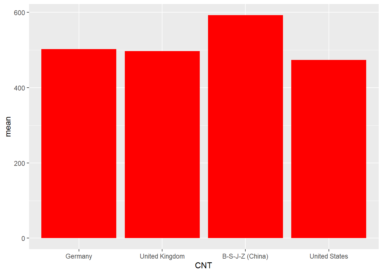
0.4 Task 4 Graphing Practice #1 A Bar Chart

Draw a bar chart of the mean mathematics scores for Germany, the UK, the US and China

Show the code

Plotdata<-PISA_2018%>%
  select(CNT, PV1MATH)%>%
  filter(CNT == "United Kingdom"| CNT == "United States"|
           CNT == "Germany"| CNT == "B-S-J-Z (China)")%>%
  group_by(CNT)%>%
  summarise(mean = mean(PV1MATH))

ggplot(Plotdata,               # Pass the data to be plotted to ggplot
       aes(x = CNT, y = mean))+    # set the x and y varibale
  geom_col(fill = "red")         # plot a column graph and fill in red

0.5 Task 5 Graphing Practice #2 A Bar Chart with two series

Draw a bar chart of the mean mathematics scores for Germany, the UK, the US and China for boys and girls

Show the code

Plotdata<-PISA_2018%>%
  select(CNT, PV1MATH, ST004D01T)%>%
  filter(CNT == "United Kingdom"|CNT=="United States"|
           CNT == "Germany"|CNT == "B-S-J-Z (China)")%>%
  group_by(CNT, ST004D01T)%>%
  summarise(mean = mean(PV1MATH))

ggplot(Plotdata,
       aes(x = CNT, y=mean, fill = ST004D01T))+ # Setting the fill to the gender
                                            # variable gives two series
  geom_col(position = position_dodge())     # position_dodge here means the

Show the code

                                            # means the bars are plotted                                                # side by side

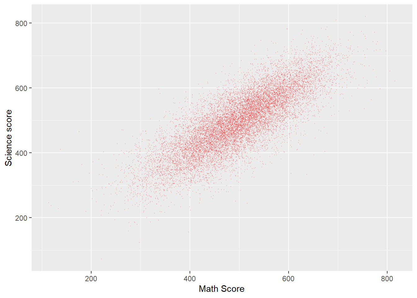
0.6 Task 6 Graphing Practice #3 A scatter plot

Plot a graph of science scores against mathematics scores for students in the UK

Show the code

Plotdata<-PISA_2018%>%              # Create a new data frame to be plotted
  select(CNT, PV1MATH, PV1SCIE)%>%  # Choose the country, and scores vectors
  filter(CNT == "United Kingdom")    # Filter for only Uk results

ggplot(Plotdata,                  # Pass the data to be plotted to ggplot
       aes(x = PV1MATH, y = PV1SCIE))+ # Define the x and y variable
      geom_point(size = 0.1, alpha = 0.2, colour="red")+ 
                                  # Use geom-point to create a scatter                                      # graph and set the size of the point 
                                    # alpha (i.e transparency)
      labs(x = "Math Score", y = "Science score") # Add clearer labels

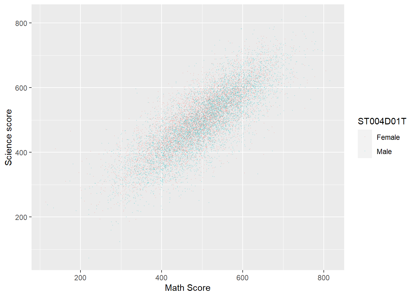
0.7 Task 7 Graphing Practice #4 A scatter plot with multiple series

Plot a graph of science scores against mathematics scores for students in the UK, with data split into two series for boys and girls

Show the code

Plotdata<-PISA_2018%>%              # Create a new dataframe to be plotted
  select(CNT, PV1MATH, PV1SCIE, ST004D01T)%>%  
  filter(CNT == "United Kingdom")    # Filter for only Uk results

ggplot(Plotdata,                  
       aes(x = PV1MATH, y = PV1SCIE, colour = ST004D01T))+ 
      geom_point(size = 0.1, alpha = 0.2)+ 
                          # As above, but set colour by the gender varibale
      labs(x = "Math Score", y = "Science score") 

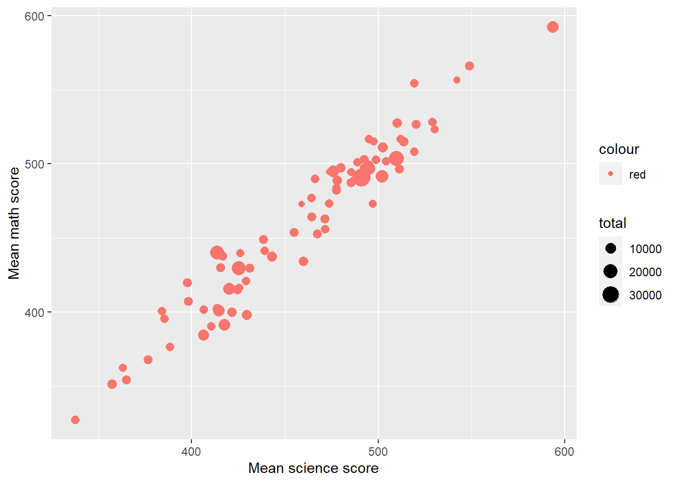
0.8 Task 8 Graphing Practice #4 A scatter plot with varying size points

Plot a graph of mean science scores against mean mathematics scores for all the countries in the data set. Vary the point size by the number of students per country.

Show the code

Plotdata<-PISA_2018%>%
  select(CNT, PV1MATH, PV1SCIE) %>%
  group_by(CNT) %>%
  summarise(meansci = mean(PV1SCIE), meanmath=mean(PV1MATH), total=n())

  # Summarise finds mean scores by countries and n() is used to sum
  # the number of students in each country

ggplot(Plotdata,
       aes(x = meansci, y = meanmath, size = total, colour = "red"))+
  # The size aesthetic is set to the total entries value computed
  # for the data set
  geom_point()+
  labs(x = "Mean science score", y = "Mean math score")

0.9 Task 9 Graphing Practice #5 A mosaic plot

Plot a mosaic plot of the number of students in general or vocational schools

Show the code

Genderschool<-PISA_2018%>%
  select(ST004D01T,ISCEDO)%>%
  filter(ST004D01T == "Male"|ST004D01T == "Female")%>%
  filter(ISCEDO == "General"|ISCEDO == "Vocational")%>%
  na.omit()%>%
  droplevels()

install.packages("ggmosaic")
library(ggmosaic)
ggplot(Genderschool)+
  geom_mosaic(aes(x = product(ST004D01T,ISCEDO), fill = ISCEDO))

0.10 Task 10 T-test practice #1

Using the PISA 2018 data set, determine if there are statistically significant differences between the science, reading and mathematics scores of the UK and the US.

Show the code

# Create data frames with the score results for UK and US
UKscores<-PISA_2018%>%
  select(CNT,PV1MATH,PV1READ, PV1SCIE)%>%
  filter(CNT == "United Kingdom")

USscores<-PISA_2018%>%
  select(CNT,PV1MATH,PV1READ, PV1SCIE)%>%
  filter(CNT == "United States")

# Perform the t-test with maths results

t.test(UKscores$PV1MATH, USscores$PV1MATH)

    Welch Two Sample t-test

data:  UKscores$PV1MATH and USscores$PV1MATH
t = 15.487, df = 8307.7, p-value < 2.2e-16
alternative hypothesis: true difference in means is not equal to 0
95 percent confidence interval:
 20.61393 26.58858
sample estimates:
mean of x mean of y 
 496.7440  473.1427 

Show the code

# p-value is < 2.2e-16 so significant differences exist for maths

t.test(UKscores$PV1READ, USscores$PV1READ)

    Welch Two Sample t-test

data:  UKscores$PV1READ and USscores$PV1READ
t = 0.19658, df = 7763.6, p-value = 0.8442
alternative hypothesis: true difference in means is not equal to 0
95 percent confidence interval:
 -3.117095  3.811951
sample estimates:
mean of x mean of y 
 500.4976  500.1502 

Show the code

# p-value = 0.8442 so no significant differences exist for reading

t.test(UKscores$PV1SCIE, USscores$PV1SCIE)

    Welch Two Sample t-test

data:  UKscores$PV1SCIE and USscores$PV1SCIE
t = -1.2472, df = 8182.1, p-value = 0.2124
alternative hypothesis: true difference in means is not equal to 0
95 percent confidence interval:
 -5.224369  1.161388
sample estimates:
mean of x mean of y 
 495.2457  497.2772 

Show the code

# p-value = 0.2124 so no significant differences exist for reading

0.11 Task 11 T-test practice #2

Divide the UK population into two groups, those that have internet access at home and those who do not. Are there statistically significant differences in the means of their reading, science and mathematics scores?

Show the code

# Create data frames with the score results for UK in two
# groups, has internet and no internet, based on ST011Q06TA

UKHasIntscores<-PISA_2018%>%
  select(CNT,PV1MATH,PV1READ, PV1SCIE, ST011Q06TA)%>%
  filter(CNT=="United Kingdom" & ST011Q06TA == "Yes")

UKNoIntscores<-PISA_2018%>%
  select(CNT,PV1MATH,PV1READ, PV1SCIE, ST011Q06TA)%>%
  filter(CNT=="United Kingdom" & ST011Q06TA == "No")

# Perform the t-test with maths results
t.test(UKHasIntscores$PV1MATH, UKNoIntscores$PV1MATH)

    Welch Two Sample t-test

data:  UKHasIntscores$PV1MATH and UKNoIntscores$PV1MATH
t = 16.181, df = 138.69, p-value < 2.2e-16
alternative hypothesis: true difference in means is not equal to 0
95 percent confidence interval:
  95.90286 122.60262
sample estimates:
mean of x mean of y 
 498.8200  389.5673 

Show the code

# p-value is < 2.2e-16 so no signficant differences for maths scores from

# those with and without internet

t.test(UKHasIntscores$PV1READ, UKNoIntscores$PV1READ)

    Welch Two Sample t-test

data:  UKHasIntscores$PV1READ and UKNoIntscores$PV1READ
t = 12.267, df = 138.04, p-value < 2.2e-16
alternative hypothesis: true difference in means is not equal to 0
95 percent confidence interval:
  82.6465 114.4084
sample estimates:
mean of x mean of y 
 503.4454  404.9180 

Show the code

# p-value is < 2.2e-16 so no signficant differences for reading scores from

# those with and without internet

t.test(UKHasIntscores$PV1SCIE, UKNoIntscores$PV1SCIE)

    Welch Two Sample t-test

data:  UKHasIntscores$PV1SCIE and UKNoIntscores$PV1SCIE
t = 14.356, df = 138.46, p-value < 2.2e-16
alternative hypothesis: true difference in means is not equal to 0
95 percent confidence interval:
  90.94524 119.99736
sample estimates:
mean of x mean of y 
 497.7262  392.2549 

Show the code

# p-value is < 2.2e-16 so no signficant differences for science scores from
# those with and without internet

0.12 Task 12 T-test practice #3

Using the PISA 2018 data set, are the mean mathematics scores of US boys and girls different to a statistically significant degree?

Show the code

# Create a dataframe of US boys math scores

USboys<-PISA_2018 %>%
  select(CNT, PV1MATH, ST004D01T)%>%
  filter(CNT == "United States")

# Create a dataframe of US girls math scores

USgirls<-PISA_2018 %>%
  select(CNT, PV1MATH, ST004D01T)%>%
  filter(CNT == "United States")

# Perform the t-test, using $PVMATH to indicate which column of the dataframe to use

t.test(USboys$PV1MATH, USgirls$PV1MATH)

    Welch Two Sample t-test

data:  USboys$PV1MATH and USgirls$PV1MATH
t = 0, df = 9674, p-value = 1
alternative hypothesis: true difference in means is not equal to 0
95 percent confidence interval:
 -3.654667  3.654667
sample estimates:
mean of x mean of y 
 473.1427  473.1427 

Show the code

# The p-value is 1 which is over 0.05 suggesting we accept the null hypothesis, there are no  statistically signficant difference in US girls and boys math scores

0.13 Task 13 T-test practice #3

Are the mean science scores of all students in the US and the UK different to a statistically significant degree?

Show the code

# Create a data frame of US science scores

USSci<-PISA_2018 %>%
  select(CNT, PV1SCIE)%>%
  filter(CNT == "United States")

# Create a data frame of UK science scores

UKSci<-PISA_2018 %>%
  select(CNT, PV1SCIE)%>%
  filter(CNT == "United Kingdom")

# Perform the t-test, using $PV1SCIE to indicate which column of the dataframe to use

t.test(USSci$PV1SCIE, UKSci$PV1SCIE)

    Welch Two Sample t-test

data:  USSci$PV1SCIE and UKSci$PV1SCIE
t = 1.2472, df = 8182.1, p-value = 0.2124
alternative hypothesis: true difference in means is not equal to 0
95 percent confidence interval:
 -1.161388  5.224369
sample estimates:
mean of x mean of y 
 497.2772  495.2457 

Show the code

# The p-value is 0.2124, over 0.05, so we accept the null hypothesis, there is no statistically significant difference between US and UK science scores  

0.14 Task 14 Chi-square practice #1

Are statiscally significant differences in the proportion of boys and girls and the number of books in the home (ST013Q01TA) for the whole dataset?

Show the code

# Create a dataframe of boys and number of books in the home

Malebooksinhome<-PISA_2018 %>%
  select(ST004D01T, ST013Q01TA)%>%
  filter(ST004D01T == "Male")

# Sum these up and convert to a data frame for chisq.test

Malebooksinhome<-as.data.frame(table(Malebooksinhome$ST013Q01TA))

# Repeat for girls

Femalebooksinhome<-PISA_2018 %>%
  select(ST004D01T, ST013Q01TA)%>%
  filter(ST004D01T == "Female")

Femalebooksinhome<-as.data.frame(table(Femalebooksinhome$ST013Q01TA))

# Perform the chisq.test

chisq.test(Malebooksinhome$Freq,Femalebooksinhome$Freq)

    Pearson's Chi-squared test

data:  Malebooksinhome$Freq and Femalebooksinhome$Freq
X-squared = 60, df = 36, p-value = 0.00727

Show the code

# The p-value is 0.00727, which is less than 0.05 so the null hypothesis, that are no signifcnat differneces between the number of boys in boys' and girls' homes is rejects. Girls and boys have different distributions of number of books.

0.15 Task 15 Chi-square practice #2

Are there statistically significant differences, in the whole data set, between boys and girls use of the internet at school to browse for homework (IC011Q03TA)?

Show the code

# Create a data frame of the girls responses to the question on internet use at school 

girlsint<-PISA_2018%>%
  select(IC011Q03TA, ST004D01T)%>%
  filter(ST004D01T == "Female")%>%
   select(IC011Q03TA)

# Do the same for boys

boysint<-PISA_2018%>%
  select(IC011Q03TA, ST004D01T)%>%
  filter(ST004D01T == "Male")%>%
   select(IC011Q03TA)

# Create frequency count tables of those data frames
# Note the chisq.test function takes data frames as inputs
# but the output of table is a table, so we convert the tables
# back to data frames

girlsint<-as.data.frame(table(girlsint))
boysint<-as.data.frame(table(boysint))

# Run the chi.sq test using the freq column in the dataframe

chisq.test(girlsint$Freq,boysint$Freq)

    Pearson's Chi-squared test

data:  girlsint$Freq and boysint$Freq
X-squared = 45, df = 25, p-value = 0.008362

Show the code

# The output p-value is 0.008362 which is less than 0.05. So reject the null hypothesis. There is a difference in usage.

0.16 Task 16 Chi-square practice #3

Are there statistically significant differences between the availability of laptops (IC009Q02TA) in school in the US and the UK?

Show the code

# IC009Q02TA - Available for use in school - a laptop
# Filter the data to get laptop use in the UK, put that into a new dataframe UKchidata

UKchidata<- PISA_2018 %>%
  select(CNT, IC009Q02TA)%>%
  filter(CNT == "United Kingdom")%>%
  select(IC009Q02TA)%>%
  na.omit()

# Filter the data to get laptop use in the US, put that into a new dataframe USchidata

USchidata<- PISA_2018 %>%
  select(CNT, IC009Q02TA)%>%
  filter(CNT == "United States")%>%
  select(IC009Q02TA)%>%
  na.omit()

# use table to count the entries and convert to a data frame

UKchidata<-as.data.frame(table(UKchidata))
USchidata<-as.data.frame(table(USchidata))

# Do the chi squared test

chisq.test(UKchidata$Freq, USchidata$Freq)

    Pearson's Chi-squared test

data:  UKchidata$Freq and USchidata$Freq
X-squared = 21, df = 9, p-value = 0.01265

Show the code

# p-value is less than 0.05, so reject the null hypotheses - there are statistically significant differences in access to laptops in the UK and the US

0.17 Task 18 Anova practice #1

Are there statistically significant differences in mathematics scores of France, Germany, Spain, the UK and Italy? Find between which pairs of countries statistically significant differences in mathematics scores exist.

Show the code

# Create a data frame of the required countries

EuroPISA <- PISA_2018 %>%
  select(CNT, PV1MATH)%>%
  filter(CNT == "Spain"| CNT == "France"| CNT == "United Kingdom"| 
         CNT == "Italy"| CNT == "Germany")

# Perform the anova

resaov<-aov(data=EuroPISA, PV1MATH ~ CNT)
summary(resaov)

               Df    Sum Sq Mean Sq F value Pr(>F)    
CNT             4   1082967  270742   33.71 <2e-16 ***
Residuals   73300 588650518    8031                   
---
Signif. codes:  0 '***' 0.001 '**' 0.01 '*' 0.05 '.' 0.1 ' ' 1

Show the code

# Yes, statistically significant differences exist between the countries Pr(>F) <2e-16 ***
# Perform a Tukey HSD test

TukeyHSD(resaov)

  Tukey multiple comparisons of means
    95% family-wise confidence level

Fit: aov(formula = PV1MATH ~ CNT, data = EuroPISA)

$CNT
                             diff        lwr        upr     p adj
Spain-Germany          -11.317134 -14.870244  -7.764024 0.0000000
France-Germany         -14.781715 -19.302215 -10.261215 0.0000000
United Kingdom-Germany  -5.263839  -9.173636  -1.354043 0.0022356
 [ reached getOption("max.print") -- omitted 7 rows ]

Show the code

# Significant differences p<0.05 exist for all countries except Italy and the UK

0.18 Task 19 Anova practice #2

For the UK PISA 2018 data set, which variable out of WEALTH, ST004D01T, OCOD1 (Mother’s occupation), OCOD2 (Father’s occupation), ST011Q06TA (having a link to the internet), and highest level of parental education (HISCED) accounts for the most variation in science score? What percentage of variance is explained by each variable?

! This is a big calculation so will take some time to compute !

Show the code

# Create a data frame for the UK
UKPISA_2018 <- PISA_2018 %>%
  filter(CNT == "United Kingdom")

# Perform the anova calculation with science score as the dependent variable

resaov<-aov(data=UKPISA_2018, PV1SCIE ~ WEALTH + ST004D01T + OCOD1 + 
              OCOD2 + ST011Q06TA + HISCED)

# Print the output
summary(resaov)

               Df   Sum Sq Mean Sq F value   Pr(>F)    
WEALTH          1  1229855 1229855 161.257  < 2e-16 ***
ST004D01T       1     4594    4594   0.602    0.438    
 [ reached getOption("max.print") -- omitted 5 rows ]
---
Signif. codes:  0 '***' 0.001 '**' 0.01 '*' 0.05 '.' 0.1 ' ' 1
1517 observations deleted due to missingness

Show the code

# Calcuate the value of eta and multiple by a 100 to get the % of variance explained
eta <- etaSquared(resaov)
eta <- 100*eta
eta <- as.data.frame(eta)
eta

                 eta.sq eta.sq.part
WEALTH     0.0274095131 0.034125604
ST004D01T  0.0009201313 0.001145967
OCOD1      5.7963046843 6.732968928
OCOD2      6.9703867564 7.987839939
ST011Q06TA 0.6896365614 0.851595309
HISCED     0.2680766101 0.332765721

Show the code

# Most variance explained by OCOD2 (father's occupation), OCOD1 (mother's occupation)  HISCED (highest level of parental education), ST011Q06TA (having an internet link), WEALTH, then ST004DO1T (gender)