Piping allows us to break down complex tasks into manageable chunks that can be written and tested one after another. There are several powerful commands in the tidyverse as part of the dplyr package that can help us group, filter, select, mutate and summarise datasets. With this small set of commands we can use piping to convert massive datasets into simple and useful results.
Using the pipe %>% command, we can feed the results from one command into the next command making for reusable and easy to read code.
how piping works
Note
The pipe command we are using %>% is from the magrittr package which is installed alongside the tidyverse. Recently R introduced another pipe |> which offers very similar functionality and tutorials online might use either. The examples below use the %>% pipe.
Let’s look at an example of using the pipe on the PISA_2018 table to calculate the best performing OECD countries for maths PV1MATH by gender ST004D01T:
# A tibble: 74 × 5
# Groups:   CNT [37]
   CNT            ST004D01T mean_maths sd_maths students
   <fct>          <fct>          <dbl>    <dbl>    <int>
 1 Japan          Male            533.     90.5     2989
 2 Korea          Male            530.    102.      3459
 3 Estonia        Male            528.     85.0     2665
 4 Japan          Female          523.     82.2     3120
 5 Korea          Female          523.     96.0     3191
 6 Switzerland    Male            520.     92.7     3033
 7 Estonia        Female          519.     76.0     2651
 8 Czech Republic Male            518.     98.0     3501
 9 Belgium        Male            518.     95.9     4204
10 Poland         Male            517.     91.8     2768
# ℹ 64 more rows
line 1 passes the whole PISA_2018 dataset and pipes it into the next line %>%
line 2 filters out any results that are from non-OECD countries by finding all the rows where OECD equals == “Yes”, this is then piped to the next line
line 3 groups the data by country CNT and by student gender ST004D01T, this is then piped to the next line
line 4-6 the summarise command performs a calculation on the country and gender groupings returning three new columns, each command on a new line and separated by a comma: the mean value for maths mean_maths, the standard deviation sd_maths and a column telling us how many students were in each grouping using the n() which returns the number of rows in a group. These new columns and the grouping columns are then piped to the next line
line 7 filters out any gender ST004D01T that is NA. First is finds all the students that have NA as their gender by using is.na(ST004D01T), then is NOTs/flips the result using the exclamation mark !, giving those students who don’t have their gender set to NA. The filtered data is then piped to the next line
line 8, finally we arrange / sort the results in descending order by the mean_maths column. The default for arrange is ascending order, leave out the desc( ) for the numbers to be ordered in the opposite way.
Males get a slightly better maths score than Females for this PV1MATH score, other scores are available, please read ?@sec-PV to find out more about the limitations of using this value.
Note
we met the assignment command earlier <-. Within the tidyverse commands we use the equals sign instead =.
The commands we have just used come from a package within the tidyverse called dplyr, let’s take a look at what they do:
command
purpose
example
select
reduce the dataframe to the fields that you specify
select(<field>, <field>, <field>)
filter
get rid of rows that don’t meet one or more criteria
filter(<field> <comparison>)
group
group fields together to perform calculations
group_by(<field>, <field>))
mutate
add new fields or change values in current fields
mutate(<new_field> = <field> / 2)
summarise
create summary data optionally using a grouping command
summarise(<new_field> = max(<field>))
arrange
order the results by one or more fields
arrange(desc(<field>))
Note
If you want to explore more of the functions of dplyr, take a look at the helpsheet
Adjust the code above to find out the lowest performing countries for reading PV1READ by gender that are not in the OECD
# A tibble: 612,004 × 4
   CNT       ESCS ST004D01T ST003D02T
   <fct>    <dbl> <fct>     <fct>
 1 Albania  0.675 Male      February
 2 Albania -0.757 Male      July
 3 Albania -2.51  Female    April
 4 Albania -3.18  Male      April
 5 Albania -1.76  Male      March
 6 Albania -1.49  Female    February
 7 Albania NA     Female    July
 8 Albania -3.25  Male      August
 9 Albania -1.72  Female    March
10 Albania NA     Female    July
# ℹ 611,994 more rows
You might also be in the situation where you want to select everything but one or two fields, you can do this with the negative signal -:
# A tibble: 612,004 × 3
   CNTSTUID CNTSCHID ST004D01T
      <dbl>    <dbl> <fct>
 1   800251   800002 Male
 2   800402   800002 Male
 3   801902   800002 Female
 4   803546   800002 Male
 5   804776   800002 Male
 6   804825   800002 Female
 7   804983   800002 Female
 8   805287   800002 Male
 9   805601   800002 Female
10   806295   800002 Female
# ℹ 611,994 more rows
With hundreds of fields, you might want to focus on fields whose names match a certain pattern, to do this you can use starts_with, ends_with, contains:
PISA_2018 %>%select(ends_with("NA"))
# A tibble: 612,004 × 19
   ST011Q16NA ST012Q05NA  ST012Q06NA ST012Q09NA ST125Q01NA ST060Q01NA ST061Q01NA
   <fct>      <fct>       <fct>      <fct>      <fct>           <dbl> <fct>
 1 Yes        <NA>        One        One        6 years o…         31 45
 2 Yes        Three or m… One        None       4 years            37 45
 3 No         One         None       None       4 years            NA 45
 4 No         <NA>        None       One        1 year or…         31 45
 5 No         One         One        None       3 years            80 100
 6 No         Three or m… One        None       6 years o…         24 25
 7 <NA>       <NA>        <NA>       <NA>       <NA>               NA <NA>
 8 No         None        None       None       1 year or…         NA 45
 9 Yes        Three or m… One        One        4 years            36 45
10 <NA>       <NA>        <NA>       <NA>       <NA>               NA <NA>
# ℹ 611,994 more rows
# ℹ 12 more variables: IC009Q05NA <fct>, IC009Q06NA <fct>, IC009Q07NA <fct>,
#   IC009Q10NA <fct>, IC009Q11NA <fct>, IC008Q07NA <fct>, IC008Q13NA <fct>,
#   IC010Q02NA <fct>, IC010Q05NA <fct>, IC010Q06NA <fct>, IC010Q09NA <fct>,
#   IC010Q10NA <fct>
When you come to building your statistical models you often need to use numeric data, you can find the columns that have only numbers in them by the following. Be warned though, sometimes there are numeric fields which have a few words in them, so R treats them as characters. Use the PISA codebook to help work out where those numbers are.
Not only does the PISA_2018 dataset have a huge number of columns, it has hundred of thousands of rows. We want to filter this down to the students that we are interested in, i.e. filter out data that isn’t useful for our analysis. If we only wanted the results that were Male, we could do the following:
# A tibble: 307,044 × 5
   CNT       ESCS ST004D01T ST003D02T PV1MATH
   <fct>    <dbl> <fct>     <fct>       <dbl>
 1 Albania  0.675 Male      February     490.
 2 Albania -0.757 Male      July         462.
 3 Albania -3.18  Male      April        483.
 4 Albania -1.76  Male      March        460.
 5 Albania -3.25  Male      August       441.
 6 Albania NA     Male      March        280.
 7 Albania -1.09  Male      March        523.
 8 Albania -1.24  Male      June         314.
 9 Albania -0.164 Male      August       428.
10 Albania -0.451 Male      December     369.
# ℹ 307,034 more rows
We can combine filter commands to look for Males born in September and where the PV1MATH figure is greater than 750. We can list multiple criteria in the filter by separating the criteria with commas, using commas mean that all of these criteria need to be TRUE for a row to be returned. A comma in a filter is the equivalent of an AND, :
# A tibble: 56 × 5
   CNT                    ESCS ST004D01T ST003D02T PV1MATH
   <fct>                 <dbl> <fct>     <fct>       <dbl>
 1 United Arab Emirates  0.861 Male      September    760.
 2 Belgium               0.887 Male      September    751.
 3 Bulgaria             -0.160 Male      September    752.
 4 Canada                1.38  Male      September    751.
 5 Canada                1.16  Male      September    760.
 6 Canada                0.760 Male      September    770.
 7 Switzerland           0.814 Male      September    783.
 8 Germany               0.740 Male      September    762.
 9 Spain                 1.46  Male      September    787.
10 Estonia               0.897 Male      September    752.
# ℹ 46 more rows
Remember to include the == sign when looking to filter on equality; additionally, you can use != (not equals), >=, <=, >, <.
Remember matching is case sensitive, “june” != “June”
Rather than just looking at September born students, we want to find all the students born in the Autumn term. But if we add a couple more criteria on ST003D02T nothing is returned!
The reason is R is looking for inidividual students born in September AND October AND November AND December. As a student can only have one birth month there are no students that meet this criteria. We need to use OR :
To create an OR in a filter we use the bar | character, the below looks for all students who are “Male” AND were born in “September” OR “October” OR “November” OR “December”, AND have a PV1MATH > 750.
# A tibble: 175 × 5
   CNT                     ESCS ST004D01T ST003D02T PV1MATH
   <fct>                  <dbl> <fct>     <fct>       <dbl>
 1 Albania               0.539  Male      October      789.
 2 United Arab Emirates  0.861  Male      September    760.
 3 United Arab Emirates  0.813  Male      October      753.
 4 United Arab Emirates  0.953  Male      November     766.
 5 United Arab Emirates  0.930  Male      November     773.
 6 United Arab Emirates  1.44   Male      October      752.
 7 Australia             1.73   Male      December     756.
 8 Australia            -0.0537 Male      October      827.
 9 Australia             1.18   Male      November     758.
10 Australia             1.13   Male      October      757.
# ℹ 165 more rows
It’s neater, maybe, to use the %in% command, which checks to see if the value in a column is present in a vector, this can mimic the OR/| command:
PISA_2018 %>%select(CNT, ESCS) %>%#1 you have ESCS in the filter, it needs to be in the select as wellfilter(CNT %in%c("France", "Belgium"), #2 Belgium needs a capital letter#3 the %in% command needs percentages#4 you need a comma (or &) at the end of the line ESCS <0)
Use filter to find all the students with Three or more cars in their home ST012Q02TA. How does this compare to those with no None cars?
Adjust your code in Q2. to find the number of students with Three or more cars in their home ST012Q02TA in Italy, how does this compare with Spain?
answer
PISA_2018 %>%select(CNT, ST012Q02TA) %>%filter(ST012Q02TA =="Three or more", CNT =="Italy")PISA_2018 %>%select(CNT, ST012Q02TA) %>%filter(ST012Q02TA =="Three or more", CNT =="Spain")
Write a filter to create a table for the number of Female students with reading PV1READ scores lower than 400 in the United Kingdom, store the result as read_low_female, repeat but for Male students and store as read_low_male. Use nrow() to work out if there are more males or females with a low reading score in the UK
answer
read_low_female <- PISA_2018 %>%filter(CNT =="United Kingdom", PV1READ <400, ST004D01T =="Female")read_low_male <- PISA_2018 %>%filter(CNT =="United Kingdom", PV1READ <400, ST004D01T =="Male")nrow(read_low_female)nrow(read_low_male)# You could also pipe the whole dataframe into nrow()PISA_2018 %>%filter(CNT =="United Kingdom", PV1READ <400, ST004D01T =="Female") %>%nrow()
How many students in the United Kingdom had no television ST012Q01TAOR no connection to the internet ST011Q06TA. HINT: use levels(PISA_2018$ST012Q01TA) to look at the levels available for each column.
Very often when dealing with datasets such as PISA or TIMSS, the column names can be very confusing without a reference key, e.g. ST004D01T, BCBG10B and BCBG11. To rename columns in the tidyverse we use the rename(<new_name> = <old_name>) command. For example, if you wanted to rename the rather confusing student column for gender, also known as ST004D01T, and the column for having a dictionary at home, also known as ST011Q12TA, you could use:
                   CNT                    gender                dictionary
 Spain               : 35943   Female        :304958   Yes           :524311
 Canada              : 22653   Male          :307044   No            : 66730
 Kazakhstan          : 19507   Valid Skip    :     0   Valid Skip    :     0
 United Arab Emirates: 19277   Not Applicable:     0   Not Applicable:     0
 Australia           : 14273   Invalid       :     0   Invalid       :     0
 [ reached getOption("max.print") -- omitted 2 rows ]
If you want to change the name of the column so that it stays when you need to perform another calculation, remember to assign the renamed dataframe back to the original dataframe. But be warned, you’ll need to reload the full dataset to restore the original names:
So far we have looked at ways to return rows that meet certain criteria. Using group_by and summarise we can start to analyse data for different groups of students. For example, let’s look at the number of students who don’t have internet connections at home ST011Q06TA:
# A tibble: 3 × 2
  ST011Q06TA student_n
  <fct>          <int>
1 Yes           543010
2 No             49703
3 <NA>           19291
Line 1 passes the full PISA_2018 to the pipe
Line 2 makes groups within PISA_2018 using the unique values of ST011Q06TA
Line 3, these groups are then passed to summarise, which creates a new column called student_n and stores the number of rows in each ST011Q06TA group using the n() command. summarise only returns the columns it creates, or are in the group_by, everything else is discarded.
What we might want to do is look at this data from a country by country perspective, by adding another field to the group_by() command, we then group by the unique combination of countries CNT and internet access ST011Q06TA, e.g. Albania+Yes; Albania+No; Albania+NA; Brazil+Yes; etc
# A tibble: 240 × 3
# Groups:   CNT [80]
   CNT                  ST011Q06TA student_n
   <fct>                <fct>          <int>
 1 Albania              Yes             5059
 2 Albania              No              1084
 3 Albania              <NA>             216
 4 United Arab Emirates Yes            17616
 5 United Arab Emirates No               949
 6 United Arab Emirates <NA>             712
 7 Argentina            Yes             9871
 8 Argentina            No              1781
 9 Argentina            <NA>             323
10 Australia            Yes            12547
# ℹ 230 more rows
summarise can also be used to work out statistics by grouping. For example, if you wanted to find out the max, mean and min science grade PV1SCIE by country CNT, you could do the following:
# A tibble: 80 × 4
   CNT                    sci_max sci_mean sci_min
   <fct>                    <dbl>    <dbl>   <dbl>
 1 Albania                   674.     417.   166.
 2 United Arab Emirates      778.     425.    86.3
 3 Argentina                 790.     418.   138.
 4 Australia                 879.     502.   153.
 5 Austria                   779.     493.   175.
 6 Belgium                   764.     502.   196.
 7 Bulgaria                  741.     426.   145.
 8 Bosnia and Herzegovina    664.     398.   152.
 9 Belarus                   799.     474.   192.
10 Brazil                    747.     407.    95.6
# ℹ 70 more rows
Important
group_by() can have unintended consequences in your code if you are saving your pipes to new dataframes. To be safe your can clear any grouping by adding: my_data %>% ungroup()
4.1 Questions
Spot the three errors with the following summarise statement
PISA_2018 %>%group(CNT)summarise(num_stus = n)
answer
PISA_2018 %>%group_by(CNT) %>%#1 group_by NOT group #2 missing pipe %>%summarise(num_stus =n()) #3 = n() not = n
Write a group_by and summarise statement to work out the mean and median cultural capital value ESCS for each student by country CNT
Using summarise work out, Yes or No, by country CNT and gender ST004D01T, whether students “reduce the energy I use at home […] to protect the environment.” ST222Q01HA. Filter out any NA values on ST222Q01HA:
Sometimes you will want to adjust the values stored in a field, e.g. converting a distance in miles into kilometres; or compute a new fields based on other fields, e.g. working out a total grade given the parts of a test. To do this we can use mutate. Unlike summarise, mutate retains all the other columns either adding a new column or changing an existing one
mutate(<field> = <field_calculation>)
The PISA_2018 dataset has results for maths PV1MATH, science PV1SCIE and reading PV1READ. We could combine these to create an overall PISA_grade, and PISA_mean:
line 2 mutate creates a new field called PV1_total made up by adding together the columns for maths, science and reading. Each column acts like a vector and adding them together is the equivalent of adding each students individual grades together, row by row. See ?@sec-vectors for more details on vector addition.
line 3 inside the same mutate statement, we take the PV1_total calculated on line 2 and divide it by 3, to give us a mean value, this is then assigned to a new column, PV1_mean.
line 4 this line selects only the fields that we are interested in, dropping the others
We can use mutate to create subsets of data in fields. For example, if we wanted to see how many students in each country were high performing readers, specified by getting a reading grade of greater than 550, we could do the following:
# A tibble: 159 × 3
# Groups:   CNT [80]
   CNT                  PV1READ_high     n
   <fct>                <lgl>        <int>
 1 Albania              FALSE         6083
 2 Albania              TRUE           276
 3 United Arab Emirates FALSE        16567
 4 United Arab Emirates TRUE          2710
 5 Argentina            FALSE        11003
 6 Argentina            TRUE           972
 7 Australia            FALSE         9311
 8 Australia            TRUE          4962
 9 Austria              FALSE         4900
10 Austria              TRUE          1902
# ℹ 149 more rows
Comparisons can also be made between different columns, if we wanted to find out the percentage of Males and Females that got a better grade in their maths test PV1MATH than in their reading test PV1READ:
# A tibble: 4 × 4
# Groups:   ST004D01T [2]
  ST004D01T maths_better      n   per
  <fct>     <lgl>         <int> <dbl>
1 Female    FALSE        176021 0.583
2 Female    TRUE         126157 0.417
3 Male      FALSE        110269 0.362
4 Male      TRUE         194178 0.638
line 2 mutate creates a new field called maths_better made up by comparing the PV1MATH grade with PV1READ and creating a boolean/logical vector for the column.
line 3 selects a subset of the columns
line 4 filters out any students that don’t have gender data ST004D01T, or where the calculation on line 2 failed, i.e. PV1MATH or PV1READ was NA
line 5 group on the gender of the student
line 6 using the group on line 5, use mutate to calculate the total number of Males and Females by looking for the number of rows in each group n(), store this as students_n
line 7 re-group the data on gender ST004D01T and whether the student is better at maths than reading maths_better
line 8 count the number of students, n in each group, as specified by line 7.
line 9 create a percentage figure for the number of students in each grouping given by line 7. Use the n value from line 8 and the students_n value from line 6. NOTE: we need to use unique(students_n) to return just one value for each grouping rather than a value for every row of the line 7 grouping
For more information on how to mutate fields using ifelse, see Section 8.1
6 arrange
The results returned by pipes can be huge, so it’s a good idea to store them in objects and explore them in the Environment window where you can sort and search within the output. There might also be times when you want to order/arrange the outputs in a particular way. We can do this quite easily in the tidyverse by using the arrange(<column_name>, <column_name>) function.
# A tibble: 612,004 × 3
   CNT             ST004D01T PV1MATH
   <fct>           <fct>       <dbl>
 1 Philippines     Female       24.7
 2 Jordan          Male         51.0
 3 Jordan          Female       61.6
 4 Mexico          Female       64.3
 5 Kazakhstan      Male         70.4
 6 Jordan          Male         70.7
 7 Bulgaria        Male         73.4
 8 Kosovo          Male         76.0
 9 North Macedonia Female       78.3
10 North Macedonia Male         81.2
# ℹ 611,994 more rows
If we’re interested in the highest achieving students we can add the desc() function to arrange:
# A tibble: 612,004 × 4
   CNT                  LANGN                  ST004D01T PV1MATH
   <fct>                <fct>                  <fct>       <dbl>
 1 Canada               Another language (CAN) Male         888.
 2 Canada               Another language (CAN) Male         874.
 3 United Arab Emirates English                Male         865.
 4 B-S-J-Z (China)      Mandarin               Female       864.
 5 Australia            English                Male         863.
 6 B-S-J-Z (China)      Mandarin               Male         861.
 7 Serbia               Serbian                Male         860.
 8 Singapore            Invalid                Female       849.
 9 Australia            Cantonese              Male         845.
10 Canada               French                 Female       842.
# ℹ 611,994 more rows
7 Bring everyting together
We know that the evidence strongly indicates that repeating a year is not good for student progress, but how do countries around the world differ in terms of the percentage of their students who repeat a year?
# A tibble: 77 × 5
# Groups:   CNT [77]
   CNT                REPEAT            student_n total   per
   <fct>              <fct>                 <int> <int> <dbl>
 1 Morocco            Repeated a  grade      3333  6666 0.5
 2 Colombia           Repeated a  grade      2746  7185 0.382
 3 Lebanon            Repeated a  grade      1580  4756 0.332
 4 Uruguay            Repeated a  grade      1657  5049 0.328
 5 Luxembourg         Repeated a  grade      1655  5168 0.320
 6 Dominican Republic Repeated a  grade      1694  5474 0.309
 7 Brazil             Repeated a  grade      3227 10438 0.309
 8 Macao              Repeated a  grade      1135  3773 0.301
 9 Belgium            Repeated a  grade      2351  8089 0.291
10 Costa Rica         Repeated a  grade      1904  6571 0.290
# ℹ 67 more rows
Line 2, filter out any NA values in the REPEAT field
Line 3, group on the country of student CNT
Line 4, create a new column total for total number of rows n() in each country CNT grouping
Line 5, select on the CNT, REPEAT and total columns
Line 6, regroup the data on country CNT and whether a student has repeated a year REPEAT, i.e. Albania+Did not repeat a grade; Albania+Repeated a grade; etc.
Line 7, using the above grouping, count the number of rows in each group n() and assign this to student_n
Line 8, for each grouping keep the total number of students in each country, as calculated on line 4. Note: unique(total) is needed here to return a single value of total, rather than a value for each student in each country
Line 9, using student_n from line 7 and the number of students per country total, from line 4, create a percentage per for each grouping
Line 10, as we have percentages for both Repeated a grade and Did not repeat a grade, we only need to display one of these. Note: that there is an extra space in this
Line 11, finally, we sort the data on the per/percentage column, to show the countries with the highest level of repeating a grade. This data is self-recorded by students, so might not be totally reliable!
Line 15, save the data to your own folder as a csv
8 Advanced topics
8.1 Recoding data (ifelse)
Often we want to plot values in groupings that don’t yet exist, for example might want to give all schools over a certain size a different colour from others schools, or flag up students who have a different home language to the language that is being taught in school. To do this we need to look at how we can recode values. A common way to recode values is through an ifelse statement:
ifelse allows us to recode the data. In the example below, we are going to add a new column to the PISA_2018 dataset (using mutate) noting whether a student got a higher grade in their Maths PV1MATH or Reading PV1READ tests. ifPV1MATH is bigger then PV1READ, the maths_better is TRUE, elsemaths_better is FALSE, or in dplyr format:
We now take this new dataset maths_data and look at whether the difference between relative performance in maths and reading is the same for girls and boys:
# A tibble: 4 × 3
# Groups:   ST004D01T [2]
  ST004D01T maths_better      n
  <fct>     <lgl>         <int>
1 Female    FALSE        176021
2 Female    TRUE         126157
3 Male      FALSE        110269
4 Male      TRUE         194178
Adjust the code above to work out the percentages of Males and Females ST004D01T in each group. Check to see if the pattern also exists between science PV1SCIE and reading PV1READ:
ifelse statements can get a little complicated when using factors (see: Section 8.2). Take this example. Let’s flag students who have a different home language LANGN to the language that is being used in the PISA assessment tool LANGTEST_QQQ. We make an assumption here that the assessment tool will be the language used at school, so these students will be learning in a different language to their mother tongue. ifLANGN equals LANGTEST_QQQ, the lang_diff is FALSE, elselang_diff is TRUE, this raises an error:
Error in `mutate()`:
ℹ In argument: `lang_diff = ifelse(LANGN == LANGTEST_QQQ, FALSE, TRUE)`.
Caused by error in `Ops.factor()`:
! level sets of factors are different
The levels in each field are different, i.e. the range of home languages is larger than the range of test languages. To fix this, all we need to do is cast the factors LANGN and LANGTEST_QQQ as characters using as.character(<field>). This will then allow the comparison of the text stored in each row:
We can now look at this dataset to get an idea of which countries have the largest percentage of students learning in a language other than their mother tongue:
Unfortunately, if you explore this dataset a little further, the language fields are don’t conform well with each other and a lot more work with ifelse will be needed before you could put together any full analysis around students who speak different langages at home and at school.
Tip
It’s possible to nest our ifelse statements, by writing another ifelse where you would have the <value_if_false>, for example we might want to give describe the type of school in England:
The types of variable will heavily influence what statistical analysis you can perform. R is there to help by assigning datatypes to each field. We have different sorts of data that can be stored:
Categorical - data that can be divided into groups or categories
Nominal - categorical data where the order isn’t important, e.g. gender, or colours
Ordinal - categorical data that may have order or ranking, e.g. exam grades (A, B, C, D) or lickert scales (strongly agree, agree, disgaree, strongly disagree)
Numeric - data that consists of numbers
Continuous - numeric data that can take any value within a given range, e.g. height (178cm, 134.54cm)
Discrete - numeric data that can take only certain values within a range, e.g. number of children in a family (0,1,2,3,4,5)
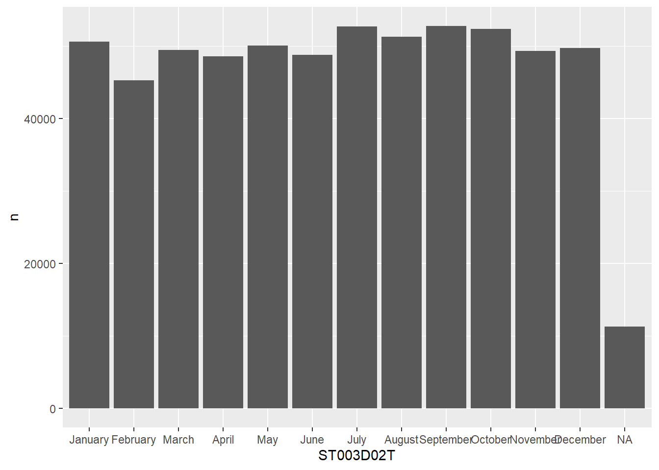
But here we are going to look at how R handles factors. Factors have two parts, levels and codes. levels are what you see when you view a table column, codes are an underlying order to the data. Factors allow you to store data that has a known set of values taht you might want to display in an order other than alphabetical. For example, if we look at the month field ST003D02T using the levels(<field>) command:
How can this be useful? A good example is how plots are made, they will use the codes to give an order to the display of columns, in the plot below, February (2) comes before March (3), even though there were more students born in March:
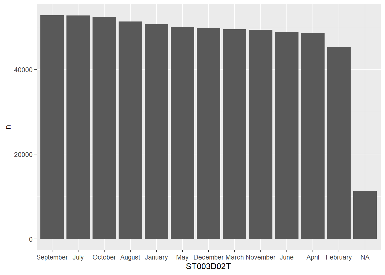
# get the levels in order and pull/create a vector of themmy_levels <- grph_data %>%arrange(desc(n)) %>%pull(ST003D02T)# reassign the re-ordered levels to the dataframe columngrph_data$ST003D02T <-factor(grph_data$ST003D02T, levels=my_levels)ggplot(data=grph_data, aes(x=ST003D02T, y=n)) +geom_bar(stat ="identity")
what is the fourth most popular language at home LANGN spoken by students in schools in the United Kingdom, how does this compare to France?
answer
PISA_2018 %>%filter(CNT %in%c("France", "United Kingdom")) %>%group_by(CNT, LANGN) %>%summarise(n =n()) %>%arrange(desc(n))# a bit of a rubbish answer really, as France only codes this at French or varieties of Other
Spot the five errors with the following code. Can you make it work? What does it do?
# Work out when more time spent in language lessons than maths lessonsPISA_2018_lang < PISA_2018 %>%rename(gender = ST004D01T) %>%mutate(language importance = LMINS - MMINS) %>%filter(is.na(language_importance)) %>%group_by(CNT gender) %>%summarise(students = n,lang_win =sum(language_importance >=0),per_lang_win =100*(lang_win/students))
answer
# Work out when more time spent in language lessons than maths lessonsPISA_2018_lang <- PISA_2018 %>%#1 make sure you have the assignment arrow <-rename(gender = ST004D01T) %>%mutate(language_importance = LMINS - MMINS) %>%#2 _ not space in name of fieldfilter(!is.na(language_importance)) %>%#3 this needs to be !is.na, otherwise it'll return nothinggroup_by(CNT, gender) %>%#4 missing commasummarise(students =n(), #5 missing brackets on the n() commandlang_win =sum(language_importance >=0),per_lang_win =100*(lang_win/students))
By gender work out the average attitudes to learning activities ATTLNACT
9.2 Teacher dataset
To further check your understanding of this section you will be attempting to analyse the 2018 teacher dataset. This dataset includes records for 107367 teachers from 19 countries, including 351 columns, covering attitudinal, demographic and workplace data. You can find the dataset here in the .parquet format.
Work out how many teachers are in the dataset for the United Kingdom
For each country CNT by gender TC001Q01NA, what is the mean time that a teacher has been in the teaching profession TC007Q02NA? Include the number of teachers in each group. Order this to show the country with the longest serving workforce: