07 Hypothesis testing and Chi-square tests
1 Pre-reading and pre-session tasks
1.1 Pre-reading
1.2 Pre-session task - Loading the data
We will continue to use the PISA_2018 dataset, make sure it is loaded.
2 Hypothesis testing
Hypothesis testing is a form of statistical inference used to draw conclusions about population distributions or parameters (such as the mean or variance). Data from a simple random sample is to test the plausibility of a hypothesis and the likelihood of it being true (or not).
When going about doing a hypothesis test we commonly choose what are called the null and alternative hypotheses. The null hypothesis usually refers to the hypothesis that there is no significant statistical difference in a set of observations, such as differences between expected values and observed values, differences between means, or differences between data and a distribution. The alternative hypothesis usually refers to the opposite of this, where there is a significant statistical difference in a set of observations, however, sometimes this can be of one direction, such as one mean being greater than another mean, instead of there being no difference.
We assume the null hypothesis is true when conducting a hypothesis test. The test itself then measures the plausibility that the null hypothesis is true and returns what is called a p-value (the probability the null hypthesis is true). If this value is relatively large then it is likely the null hypothesis is true. However, if this value is relatively small, then it is unlikely the null hypothesis is true and therefore likely it is false and that the alternative hypothesis is true instead.
Typically, we use a set value such as 0.05 or 0.01 as the threshold to determine whether the null-hypothesis is true or not. So, if the null hypothesis is greater than this value then we accept that it is true, and if it is less than this value we reject that it is true and accept that the alternative hypothesis is true instead.
2.1 Choosing a Hypotheis Test
When conducting a hypothesis test we need to choose the most appropriate test depending on the type of data we are working with, what we are trying to test and whether certain conditions are met or not. Here is a basic summary of what you may need to consider.
Type(s) of data:
Categorical (ordinal, nominal, binary);
Quantitative (continuous, discrete).
What you are trying to test:
Relationships between variables;
Comparison of means.
Distribution of data:
Normally distributed (parametric tests);
Not normally distributed (nonparametric tests).
When we consider each of the types of tests the conditions for the test will be stated, so it will be clear which test can be used when.
2.2 Performing a hypothesis test - Fisher
Fisher, one of the statisticians who moved the field of hypothesis testing forward and formalised some of the procedures used for hypothesis testing suggests using the following steps when conducting hypothesis testing.
-
Select an appropriate test.
Here, we need to consider the type(s) of data, what we are trying to test and whether the data is normally distributed or not, along with other conditions needed for the different tests.
-
Set up the null and alternative hypotheses.
This heavily depends on which test is being used, so more guidance will be given under each of the tests.
-
Calculate the theoretical probability of the null hypothesis being true.
This is where the test itself is used to calculate the probability of the null hypothesis being true (i.e. returning the p-value from the test).
-
Assess the statistical significance of the result.
This is where the p-value from step 3 is compared with a predetermined threshold, such as 0.05 or 0.01 to determine if the null hypothesis is true or false.
-
Interpret the statistical significance of the results.
Here, we take the result from step 4, so deciding whether to accept the null hypothesis or reject the null hypothesis and accept the alternative hypothesis and then what this means in the context of the problem being posed.
3 Chi-square tests
Chi squared (\(\chi^2\)) tests are non-parametric tests, this means that the test isn’t expecting the underlying data to be distributed in a certain way. Chi-squared determines how well the frequency distribution for a sample fits the population distribution and will let you know when things aren’t distributed as expected. For example you might expect girls and boys to have the same coloured dogs, a chi squared test can tell you whether the null hypothesis, that there is no difference between the colours of dogs owned by girls and boys, is true or not.
In more mathematical terms, chi squared examines differences between the categories of an independent variable with respect to a dependent variable measured on a nominal (or categorical) scale. A nominal scale has values that aren’t ordered, or continuous, for example gender or favourite flavour of ice cream.
3.1 Conditions of Chi-Square Tests
Four assumptions need to be met in order to use a chi-square test:
a) The data (both variables) should be categorical (for ordinal data, see the section on Kruskal Wallis tests below);
b) All observations are independent;
c) Cells in the contingency table (see below) are mutually exclusive;
d) Expected values in each cell in the contingency table should be five or greater for more than 80% of cells.
See Section 12.5 in Navaro’s Learning Statistics with R
3.2 Types of Chi-Square Tests
Chi-square tests can be categorised in two groups:
A test of goodness of fit - this is a form of hypothesis test which determines whether a sample fits a wider population. For example, does the pattern of exam results in one school fit the national distribution?
A test of independence - allows inference to be made about whether two categorical variables in a population are related. For example, are there differences in the uptake of careers by gender?
For more information on chi-square tests, see chapter 12, in Navaro’s Learning Statistics with R.
4 Performing chi square tests
4.1 Creating contingency tables
Chi-square calculations depend on contingency tables. A contingency table is a table that shows the frequency counts for two variables. We can use the xtabs function to create contingency tables in R.
For example, imagine we want to create a contingency table for the number of boys and girls in the UK and US in the PISA sample. First we create a subset of the PISA_2018 data.frame including country and gender, and filter for the two countries. We use the xtabs function to create the table. We pass the subset data (UKUSgender) to xtabs and indicate the columns and rows we want ~CNT + ST004D01T
# Example contingency table

UKUSgender <- PISA_2018 %>%
  select(CNT, ST004D01T) %>% # Select gender and country variables
  filter(CNT=="United Kingdom"|CNT=="United States") %>% # Filter for  UK and the US
  droplevels() # To prevent the levels for other countries confusing the table

ContTable<-xtabs(data=UKUSgender, ~CNT + ST004D01T)
ContTable
ST004D01T
CNT Female Male
United Kingdom 6996 6822
United States 2376 24625 Chi-square goodness of fit tests
If we want to determine if a sample categorical data matches the pattern of a whole population we can use a Chi-square goodness of fit test. The test is a form of hypothesis testing.
Hypothesis testing is one type of statistical analysis. A researcher states an assumption that they want to test.
For example, they might want to examine whether the distribution of boys and girls in the UK matches the expected distribution of 50:50.
A researcher typically proposes a null hypothesis - that is that there is no difference in groups. Whilst this is typical practice, and we will follow it in this course, researchers have pointed out that it is rare for the null hypothesis to be true, which impacts the validity of the test (see: Cohen (1994)) . Nonetheless, we will adopt the practice here, as it is a widely used approach.
Our null hypothesis then is:
There is no difference in the distribution of boys and girls in the UK and a random sample of 50/50 girls and boys.
Notice the ‘goodness of fit’ element - we are checking if some categorical data from a sample population (the UK) fits an expected pattern.
The outcome of a hypothesis test is typical reported by stating the value of some test (the test statistic, in this case, the Chi-squared statistic) which is used to calculate a significance level (or p-value). The p-value is the probability of obtaining test results at least as extreme as the result actually observed, under the assumption that the null hypothesis is correct.
This assumption has been critiqued, but in many research traditions, if the p-value is less than 0.05 (p>0.05) the result is taken to be statistically significant.
In the case of a Chi-squared goodness of fit test:
• If the p-value is greater than 0.05 (p<0.05) we accept the null hypothesis that the sample has been drawn from the wider population.
• If the p-value is less than 0.05 (p>0.05) we reject the null hypothesis that the sample has been drawn from the wider population.
It is important that care is taken when interpreting p-values. A p-value of below 0.05 does not mean the null hypothesis is false. Monya Baker provided a helpful summary of how to think of p-values:
“A P value of 0.05 does not mean that there is a 95% chance that a given hypothesis is correct. Instead, it signifies that if the null hypothesis is true, and all other assumptions made are valid, there is a 5% chance of obtaining a result at least as extreme as the one observed. And a P value cannot indicate the importance of a finding; for instance, a drug can have a statistically significant effect on patients’ blood glucose levels without having a therapeutic effect.”
See Baker (2016) for further discussion of how to interpret p-values.
5.1 An example: Does the disritbution of male and female students in the UK fit the expected pattern (50:50)?
To perform the goodness of fit test, we make a subset dataframe of the UK data including the ST004D01T (gender variable).
# Perform a chi-square goodness of fit test on categorical data related to gender in the UK

UKPISAgender<-PISA_2018%>%
  select(CNT, ST004D01T)%>% # Select gender and country variables
  filter(CNT=="United Kingdom")%>% # Filter for the UK
  droplevels() # To prevent the levels for other countries confusing the table

GenderContTable<-xtabs(data=UKPISAgender,~CNT + ST004D01T)

chisq.test(GenderContTable, p=c(1/2,1/2))
The outcome of the chi squared test returns a p-value = 0.1388. This is greater than 0.05, suggesting we reject the null hypothesis, and the numbers of boys and girls in the UK sample does not match a 50:50 distribution.
5.2 An example: Gender distribution in the PISA sample
- Should we accept or reject the hypothesis that the populations of boys and girls in the United States, Japan and China are 50:50?
Show the code
# Perform a chi-square goodness of fit test on categorical data related to gender in the US, Japan and China

USPISAgender<-PISA_2018%>%
  select(CNT, ST004D01T)%>% # Select gender and country variables
  filter(CNT=="United States")%>% # Filter for the US
  droplevels() # To prevent the levels for other countries confusing the table

GenderContTable<-xtabs(data=USPISAgender,~CNT + ST004D01T)

chisq.test(GenderContTable, p=c(1/2,1/2))

# In the US, population of M:F differs from 50:50 p= 0.2163, reject null hypothesis of equality.

JPNPISAgender<-PISA_2018%>%
  select(CNT, ST004D01T)%>% # Select gender and country variables
  filter(CNT=="Japan")%>% # Filter for the Japan
  droplevels() # To prevent the levels for other countries confusing the table

GenderContTable<-xtabs(data=JPNPISAgender,~CNT + ST004D01T)

chisq.test(GenderContTable, p=c(1/2,1/2))

# In Japan, population of M:F differs from 50:50 p= 0.09373, reject null hypothesis of equality.

ChinaPISAgender<-PISA_2018%>%
  select(CNT, ST004D01T)%>% # Select gender and country variables
  filter(CNT=="B-S-J-Z (China)")%>% # Filter for China
  droplevels() # To prevent the levels for other countries confusing the table

GenderFreqTable<-xtabs(data=ChinaPISAgender,~CNT + ST004D01T)

chisq.test(GenderFreqTable, p=c(1/2,1/2))
# In China, population of M:F is 50:50 p= 3.724e-06, accept null hypothesis of equality.R uses standard form: an output of p= 3.724e-06, represents, p=3.724x10⁻⁶, or p=0.0000003724.
6 Chi-square test of independence
Goodness of fit tests can be useful, but they rely on knowing the expected distribution (for example, assuming a 50:50 distribution of boys and girls).
An alternative ways of using a Chi-square test, is the test of independence. This approach determines whether two categorical variables in a sample are related.
For example, a categorical variable in the same is item - ST011Q04TA - is there a a quiet place to study in the home? Which can be responded to with ‘yes’ or ‘no’ (or <NA>).
We might want to see if students in the UK respond to this question in the same way as the rest of the sample. That is, are students in the UK just as likely to have a quiet place to study as their international peers.
A simple first attempt is to create frequency tables for the UK and the rest of the sample and examine the responses.
# Produce tables of counts of having a quiet room for the UK and the rest of the sample

QuiRoom<-PISA_2018%>%
  select(ST011Q04TA)%>% # Select quiet room
  droplevels() # To prevent the levels for other countries confusing the table

QuiFreqTable<-xtabs(data=QuiRoom,~ST011Q04TA)
print(QuiFreqTable)

UKQuiRoom<-PISA_2018%>%
  select(CNT, ST011Q04TA)%>% # Select quiet room and country variables
  filter(CNT=="United Kingdom")%>% # Filter for the UK
  droplevels() # To prevent the levels for other countries confusing the table

UKQuiFreqTable<-xtabs(data=UKQuiRoom,~ST011Q04TA)
print(UKQuiFreqTable)
From the data, it is hard to tell if the UK is different from the overall pattern. To make things easier, we can use mutate to add a percentage column to aid comparison.
# Produce tables of counts of having a quiet room for the UK and the rest of the sample

QuiRoom<-PISA_2018%>%
  select(ST011Q04TA)%>% # Select quiet room
  droplevels() # To prevent the levels for other countries confusing the table

QuiFreqTable<-xtabs(data=QuiRoom,~ST011Q04TA)
QuiFreqTable<-as.data.frame(QuiFreqTable)
Total=sum(QuiFreqTable$Freq) # Find the total count
QuiFreqTable<-QuiFreqTable%>%
  mutate(Perc=(Freq*100)/Total) # Mutate the table to calculate the percentage
print(QuiFreqTable)

UKQuiRoom<-PISA_2018%>%
  select(CNT, ST011Q04TA)%>% # Select quiet room and country variables
  filter(CNT=="United Kingdom")%>% # Filter for the UK
  droplevels() # To prevent the levels for other countries confusing the table

UKQuiFreqTable<-xtabs(data=UKQuiRoom,~ST011Q04TA)
UKQuiFreqTable<-as.data.frame(UKQuiFreqTable)
Total=sum(UKQuiFreqTable$Freq) # Find the total count
UKQuiFreqTable<-UKQuiFreqTable%>%
  mutate(Perc=(Freq*100)/Total)  # Mutate the table to calculate the percentage
print(UKQuiFreqTable)
6.1 Plotting the chi-square relationships
The numbers in the contingency table are hard to interpret - it is challenging to see how far out the numbers for each row are from each other. Alternatively, we can visualise the data from the contingency table by building a mosaic plot, a form of stacked bar chart. Mosaic plots can be a useful visulations before running a chi-squared test.
To create a mosaic plot, you are going to need to install and load the ggmosaic package. See ?@sec-load-run-pckges for more details on how to do this.
Imagine we want to plot the ‘quiet room’ data (ST011Q04TA) from the previous section for the UK, US, and Brazil
To create the mosaic plot we use ggplot, as we used for previous graphs. As before, we first pass the data (in this case QuiRoom) to ggplot. Then, to create the graph, geom_mosaic is used. geom_mosaic does not have a direct mapping of input to x and y variable so we need to pass it what we want plotted on the y-axis (ST011Q04TA) and x-axis (CNT) within the product function (product(ST011Q04TA, CNT)). We can also specify how we want the rectangles to be coloured (in our case, by CNT).
 # install.packages("ggmosaic")
library(ggmosaic)

QuiRoom<-PISA_2018%>%
  select(ST011Q04TA, CNT)%>%
  filter(CNT=="United Kingdom" | CNT=="Brazil"| CNT=="United States")%>%
  droplevels()

# plot results
ggplot(data = QuiRoom) +
  geom_mosaic(aes(x = product(ST011Q04TA, CNT), fill=CNT))+
  xlab("Country")+
  ylab("Do you have a quiet room to work in?")
6.2 Running Chi-square tests of independence
The mosaic plot suggests the availability of quiet rooms is different between the UK and Brazil, but the difference is only small between the UK and the US. Simply looking at the data does not tell us if the distributions are different - a Chi-square tests of independence can report the significance level, which can help us make a judgement.
The null hypothesis in a test of independence is that the categorial variables are not related. So in the case of comparing the UK and Brazil the null hypothesis is: ‘There is no relationship between the country (UK or Brazil) and availability of a quiet room’.
# Produce tables of counts of having a quiet room for the UK and the rest of the sample

BraUKQuiRoom<-PISA_2018%>%
  select(ST011Q04TA, CNT)%>% # Select quiet room
  filter(CNT=="Brazil"| CNT=="United Kingdom")%>% # Filter for Brazil and UK
  droplevels() # To prevent the levels for other countries confusing the table

BraUKQuiFreqTable<-xtabs(~ST011Q04TA+CNT, data=BraUKQuiRoom)

UKUSQuiRoom<-PISA_2018%>%
  select(CNT, ST011Q04TA)%>% # Select quiet room and country variables
  filter(CNT=="United Kingdom"|CNT=="United States")%>% # Filter for the UK
  droplevels() # To prevent the levels for other countries confusing the table

UKUSQuiFreqTable<-xtabs(~ST011Q04TA+CNT, data=UKUSQuiRoom)

# Perform Chisq test between UK and Brazil
chisq.test(BraUKQuiFreqTable)
# p-value < 2.2e-16, less than 0.05, so there are signifcant differences by UK and Brazil, the null hypothesis is rejected
# Perform Chisq test between UK and US
chisq.test(UKUSQuiFreqTable)
# p-value = 1.924e-15 less than 0.05, so there are signifcant differences by UK and Brazil, the null hypothesis is rejected
The test here returns a p-value=1. This is more than 0.05 so implies there is a the null hypothesis can be accepted. The null hypothesis is that and it is assumed that the availability of quiet rooms in the UK is different from the population as a whole.
7 Testing ordinal data - the Kruskal Wallis test
An assumption of a chi-square test is that the data are categorical. Some of the items in the PISA are a type of categorical data which come in naturally ordered sequence - ordinal data. For example, gender is a categorical variable with no preferred order to responses: female or male. By contrast, the answer to a question: How many books do you have in your home? 0-10; 11-100; 101-200; More than 200, is ordinal data.
Though there is some debate among statisticians, but if testing ordinal data, it is recommend you use an alternative to the chi-square test, the Kruskal Wallis test, which functions in a similar manner. It is called using the kruskal.test function. Unlike the chi square test, you pass it the raw data, rather than a contingency table.
For example,ST012Q02TA asks students to report the number of cars in their home, ordinal data. To carry out the Kruskal Wallis on differences in car ownership in the UK by gender we create a data.frame of responses to ST012Q02TA in the UK by gender. Unlike the chi square test, there is no need to create a contingency table and we just pass the data frame to kruskal.test, specifiying we want to compare number of cars (ST012Q02TA) to gender (ST004D01T): kruskal.test(data=CarsUKGender,ST012Q02TA~ST004D01T)
CarsUKGender<-PISA_2018%>%
  select(CNT, ST004D01T,ST012Q02TA )%>% # choose country, no of cars and gender
  filter(CNT=="United Kingdom")%>% # filter for the UK
  select(ST004D01T,ST012Q02TA )%>% #drop the country variable now filtering is done
  droplevels() # Remove other countries which exist as factors
# Make the contingency table

kruskal.test(data=CarsUKGender,ST012Q02TA~ST004D01T) # Perform the test
    Kruskal-Wallis rank sum test

data:  ST012Q02TA by ST004D01T
Kruskal-Wallis chi-squared = 1.8514, df = 1, p-value = 0.17368 Seminar Tasks
8.1 Task 1 - Creating contingency tables
- Create a contingency table for UK, Germany and France levels of maternal education (
ST005Q01TA). In which countries are most mothers (in total) educated to post school level?
The responses to ST005Q01TA are:
- ISCED level 3A
- Post-16 technical equivalents
- ISCED level 3B, 3C
- A-level equivalents
- ISCED level 2
- Lower secondary education ISCED level 1
- Primary Education She did not complete ISCED Level 1
- Did not complete primary education
Show the code
# Create contingency table of mother's level of education

MatEd<-PISA_2018%>%
  select(CNT, ST005Q01TA)%>% # Select maternal ed and country variables
  filter(CNT=="United Kingdom"| CNT=="France"|CNT=="Germany")%>% # Filter for CNT
  droplevels() # To prevent the levels for other countries confusing the table

ContTab<-xtabs(~ST005Q01TA +CNT, data=MatEd)
ContTab
CNT
ST005Q01TA Germany France United Kingdom
ISCED level 3A 1590 3501 6024
ISCED level 3B, 3C 400 1559 4991
ISCED level 2 2025 711 670
ISCED level 1 14 91 92
She did not complete ISCED level 1 233 159 100-
ST011Q01TAasks if students have a desk to study at. Create a contingency table by gender for this variable for students in the UK. Do more girls or boys have a desk?
Show the code
# Create contingency table of having a desk to study at

DeskUK <- PISA_2018 %>%
  select(CNT, ST011Q01TA, ST004D01T) %>% # Select desk and country variables
  filter(CNT=="United Kingdom") %>% # Filter for the UK
  droplevels() # To prevent the levels for other countries confusing the table

ContTab<-xtabs(~ST011Q01TA + ST004D01T, data=DeskUK)

ContTab
ST004D01T
ST011Q01TA Female Male
Yes 5968 5728
No 763 745-
ST011Q06TAasks if students have access to the internet. In which country in the data frame do students report the highest levels of access to the internet?
To sort a table, the easiest way is to convert it to a dataframe and then use the arrange function. The default order for arrange is ascending, adding desc switches to descending.
# Arranging a table

PISA_2018 %>%
  select(CNT, ST011Q06TA) %>% # Select internet and country variables
  filter(ST011Q06TA == "Yes") %>%
  group_by(CNT) %>%
  count() %>%
  arrange(desc(n))
# A tibble: 80 × 2
# Groups: CNT [80]
CNT n
<fct> <int>
1 Spain 34663
2 Canada 21116
3 United Arab Emirates 17616
4 Kazakhstan 17511
5 United Kingdom 13126
6 Qatar 12613
7 Australia 12547
8 B-S-J-Z (China) 11286
9 Italy 11127
10 Argentina 9871
# ℹ 70 more rows8.2 Task 2 - Goodness of fit test. Are the responses of the survey in proportion to populations?
The populations of three countries in the sample are:
| Country | Population | Ratio |
|---|---|---|
| US | 332 million | 0.69 |
| Germany | 83 million | 0.17 |
| UK | 67 million | 0.14 |
Are the number of responses in the sample a good fit for the overall populations?
Use a goodness of fit implementation of Chi square with the null hypothesis that the proportion of students in the sample of PISA match that of the overall population. Hint: You can use the CNT column to create counts of the total data.
8.3 Task 3 - Goodness of fit test: Birth month distribution
Perform a goodness of fit test to determine if the birth months (ST003D02T) of respondents are distributed as expected in
- the whole sample;
- in the UK. Use ggplot to plot a column graph of both data sets (the world and the UK).
- What might explain any patterns you see.
Show the code
Worldmonth <- PISA_2018 %>%
  select(ST003D02T) %>%
  droplevels()

Worldmonth <- as.data.frame(table(Worldmonth))

Expected <- c(rep(1/12, times=12))

chisq.test(Worldmonth$Freq, p=Expected)

# p-value < 2.2e-16, which is less than 0.05, reject the null hypothesis.The world data does not follow the expect distribution

UKmonth <- PISA_2018 %>%
  select(ST003D02T, CNT) %>%
  filter(CNT=="United Kingdom") %>%
  select(ST003D02T) %>%
  droplevels()

UKmonth <- as.data.frame(table(UKmonth))

Expected <- c(rep(1/12, times=12))

chisq.test(UKmonth$Freq, p=Expected)

# p-value < 2.2e-16, which is less than 0.05, reject the null hypothesis.The world data does not follow the expect distribution

ggplot(data=Worldmonth,
       aes(x=ST003D02T, y=Freq, fill=ST003D02T)) +
  geom_col() +
  ggtitle("World birth months")

ggplot(data=UKmonth,
       aes(x=ST003D02T,y=Freq, fill=ST003D02T)) +
  geom_col() +
  ggtitle("UK birth months")
8.4 Task 4 - Country differences - hypothesis testing
Perform a hypothesis test to determine:
-
ISCEDOcontains information about the type of school students attend - responses can be: General, Pre-Vocational, Vocational or Modular. Determine if the attendance at such schools is equivalent in the United Kingdom, United States, France, and Germany.
Plot a mosaic plot of the proportions
Show the code
SchTypes <- PISA_2018 %>%
  select(CNT, ISCEDO) %>% # choose country and type of school
  filter(CNT=="United Kingdom"|CNT=="United States"|
           CNT== "France"|CNT=="Germany")%>% # filter by four countries
  droplevels() # Remove other countries which exist as factors

# Create a contingency table
SchCont<-xtabs(data=SchTypes, ~ISCEDO+CNT)

chisq.test(SchCont) # Perform the test
# The p-value is less than 0.05 (p-value < 2.2e-16), therefore we reject the null hypothesis that the distributions are the same

ggplot(data=SchTypes) +
geom_mosaic(aes(x=product(ISCEDO,CNT), fill=ISCEDO))- Are there significant differences between Japan, Greece and the UK in
IC001Q01TA, Available for you to use at home: Desktop computer? (Yes or No). Produce a mosaic plot.
Show the code
Desktop <- PISA_2018 %>%
  select(CNT, IC001Q01TA) %>% # choose country and use of computer
  filter(CNT=="United Kingdom"|CNT=="Japan"| CNT=="Greece") %>% # filter by countries
  droplevels() # Remove other countries which exist as factors

# Produce a contingency table
ContDesk <- xtabs(data=Desktop, ~CNT+IC001Q01TA)

chisq.test(ContDesk) # Perform the test
# The p-value is less than 0.05 (p-value < 2.2e-16), therefore we reject the null hypothesis that the distributions are the same

ggplot(data=Desktop) +
  geom_mosaic(aes(x=product(IC001Q01TA,CNT), fill=IC001Q01TA))
Perform a hypothesis test to determine if ST007Q01TA - the highest level of schooling completed by respondents’ fathers, is different in the UK, US, France and Germany.
Plot a mosaic plot of the proportions.
Follow up question: Are the proportions of paternal education different in the three European countries (UK, France and Germany)?
Hint: assume the null hypothesis is that fathers have the same level of qualifications in the four countries.
Show the code
PatEdTypes<-PISA_2018%>%
  select(CNT, ST007Q01TA)%>% # choose country and type of school
  filter(CNT=="United Kingdom"|CNT=="United States"|
           CNT== "France"|CNT=="Germany")%>% # filter by four countries
  droplevels() # Remove other countries which exist as factors

Conttable<-xtabs(data=PatEdTypes,~CNT,ST007Q01TA)
chisq.test(Conttable) # Perform the test
# The p-value is less than 0.05 (p-value < 2.2e-16), therefore we reject the null hypothesis that the distributions are the same

# Create a geom_mosaic
ggplot(data=PatEdTypes)+
  geom_mosaic(aes(x=product(ST007Q01TA,CNT), fill=ST007Q01TA))+
  ylab("Frequency of father's level of qualification")+
  xlab("Country")+
  theme(axis.text.x = element_text(angle = 90, vjust = 0.5, hjust=1))# Rotate x-axis labels

# Follow up Question

PatEdTypes<-PISA_2018%>%
  select(CNT, ST007Q01TA)%>% # choose country and type of school
  filter(CNT=="United Kingdom"|CNT== "France"|CNT=="Germany")%>%
  droplevels() # Remove other countries which exist as factors

Conttable<-xtabs(data=PatEdTypes,~CNT,ST007Q01TA)
chisq.test(Conttable) # Perform the test
# The p-value is less than 0.05 (p-value < 2.2e-16), therefore we reject the null hypothesis that the distributions are the same

# Create a geom_mosaic
ggplot(data=PatEdTypes)+
  geom_mosaic(aes(x=product(ST007Q01TA,CNT), fill=ST007Q01TA))+
  ylab("Frequency of father's level of qualification")+
  xlab("Country")+
  theme(axis.text.x = element_text(angle = 90, vjust = 0.5, hjust=1))# Rotate x-axis labels
9 Testing ordinal data with the Kruskal-Wallis test
Are there differences in the number of books in the homeST013Q01TA in the UK and the United States? Create a mosaic plot
Show the code
    Kruskal-Wallis rank sum test

data:  ST013Q01TA by CNT
Kruskal-Wallis chi-squared = 149.18, df = 1, p-value < 2.2e-16
Show the code
# The p-value is more than 0.05 (p-value=1), therefore we accept the null hypothesis that the number of books is the same for respondents in the UK and the US

# Create a geom_mosaic
ggplot(data=UKUSbooks)+
  geom_mosaic(aes(x=product(ST013Q01TA,CNT), fill=ST013Q01TA))+
  ylab("Number of books in the home")+
  xlab("Country")+
  theme(axis.text.x = element_text(angle = 90, vjust = 0.5, hjust=1))# Rotate x-axis labels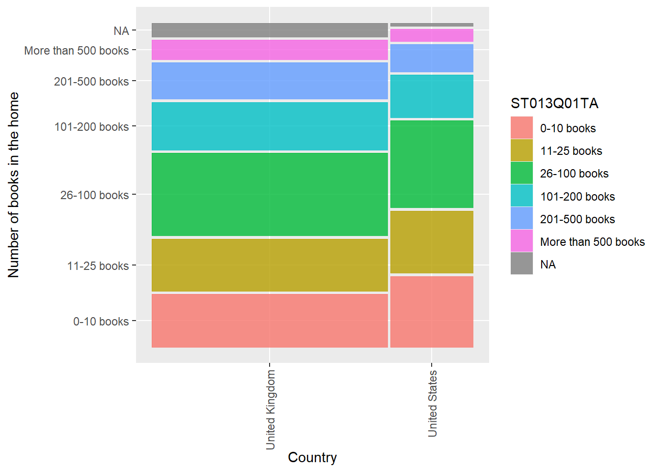
In the UK, are there differences for boys and girls for the number of instruments in the home (ST012Q09NA)? Create a mosaic plot.
Show the code
UKInstruments<-PISA_2018%>%
  select(CNT, ST012Q09NA, ST004D01T )%>% # choose CNT, no of instruments, gender
  filter(CNT=="United Kingdom")%>% # filter for the UK
  select(ST012Q09NA, ST004D01T)%>% #drop the country variable now filtering is done
  droplevels() # Remove other countries which exist as factors
# Make the contingency table
kruskal.test(UKInstruments,ST012Q09NA ~ST004D01T) # Perform the test
    Kruskal-Wallis rank sum test

data:  UKInstruments
Kruskal-Wallis chi-squared = 21197, df = 1, p-value < 2.2e-16
Show the code
# The p-value is less than 0.05 (p-value < 2.2e-16), therefore we reject the null hypothesis. Girls and boys have different access to instruments in the home.

# Create a geom_mosaic
ggplot(data=UKInstruments)+
  geom_mosaic(aes(x=product(ST012Q09NA,ST004D01T), fill=ST012Q09NA))+
  ylab("Number of instruments in the home for UK young people")+
  xlab("Gender")+
  theme(axis.text.x = element_text(angle = 90, vjust = 0.5, hjust=1))# Rotate x-axis labels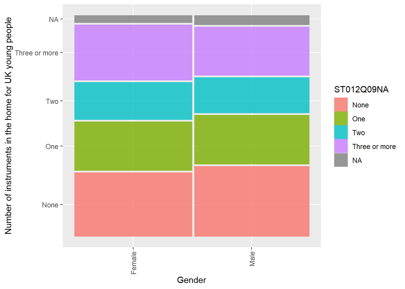
In the UK, are there differences for boys and girls in the number of smart phones in the home (ST012Q05NA)? Plot the data as a mosaic plot.
Show the code
UKPhones<-PISA_2018%>%
  select(CNT, ST012Q05NA, ST004D01T )%>% # choose CNT, no of instruments, gender
  filter(CNT=="United Kingdom")%>% # filter for the UK
  select(ST012Q05NA, ST004D01T)%>% #drop the country variable now filtering is done
  droplevels() # Remove other countries which exist as factors
# Make the contingency table
kruskal.test(UKPhones,ST012Q05NA ~ST004D01T) # Perform the test
    Kruskal-Wallis rank sum test

data:  UKPhones
Kruskal-Wallis chi-squared = 23239, df = 1, p-value < 2.2e-16
Show the code
# The p-value is less than 0.05 (p-value < 2.2e-16), therefore we reject the null hypothesis. Girls and boys have different access to phones in the home.

# Create a geom_mosaic
ggplot(data=UKPhones)+
  geom_mosaic(aes(x=product(ST012Q05NA,ST004D01T), fill=ST012Q05NA))+
  ylab("Number of phones in the home for UK young people")+
  xlab("Gender")+
  theme(axis.text.x = element_text(angle = 90, vjust = 0.5, hjust=1))# Rotate x-axis labels
10 Extension tasks
Whilst chi-square tests are useful for reporting whether there are significant differences between the distribution of values in a contingency table, they don’t, by themselves tell you which cells in the contingency table differ from the expected values. To find out this information, you can do a post-hoc analysis. For example, if we want to consider if there are differences in the distribution of school types (ISCEDO - i.e general, vocational, etc) we create a subset of PISA data for the the UK, US, France and Germany (PISAsub), create a contingency table, plot the data, and perform the chisq.test.
PISAsub<-PISA_2018%>%
  select(CNT, ISCEDO)%>% # choose country and type of school
  filter(CNT %in% c("United Kingdom", "United States", "France", "Germany"))%>% # filter by four countries
  droplevels() # Remove other countries which exist as factors

ContTab<-(xtabs(~CNT + ISCEDO, PISAsub)) # Create contingency table by CNT and school type

ggplot(data=PISAsub)+
  geom_mosaic(aes(x=product(ISCEDO, CNT), fill=ISCEDO))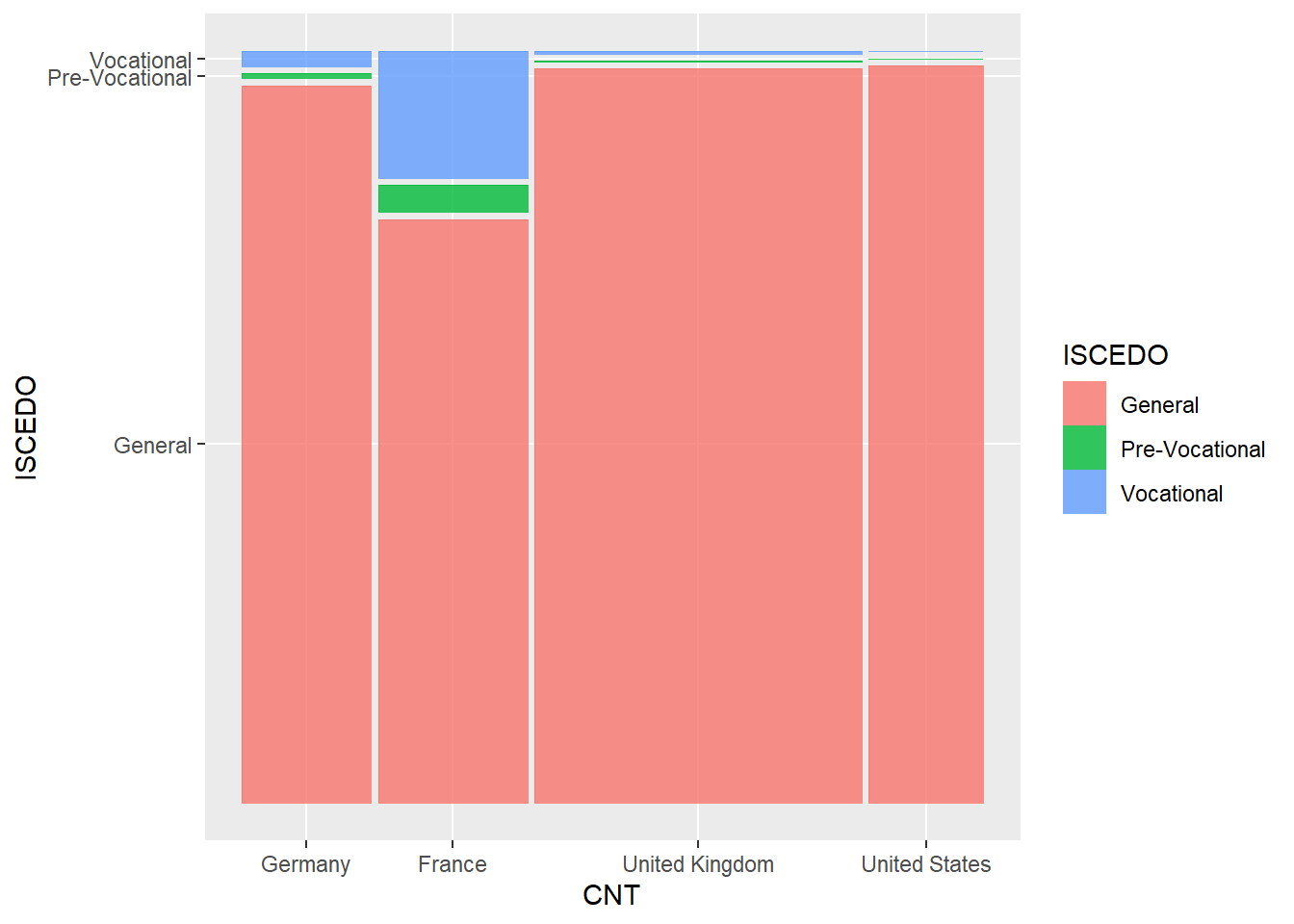
    Pearson's Chi-squared test

data:  ContTab
X-squared = 4281.8, df = 6, p-value < 2.2e-16 Dimension Value General Pre-Vocational Vocational
1 Germany Residuals 8.654495 -2.485784 -8.333644
2 Germany p values 0.000000 0.155120 0.000000
3 France Residuals -65.021954 26.206030 58.987616
[ reached 'max' / getOption("max.print") -- omitted 5 rows ]In this case, the chi square test returns a p-value < 2.2e-16 suggesting significant differences between the countries.We can use the package chisq.posthoc.test to use the function chisq.posthoc.test to perform the additional test.
The posthoc test returns a table of residuals and p-values for each cell in the contingency table The residuals give a sense how much each cell contributes to the total chi-squared value. The right most column (Pr(>Chi)) reports whether this deviation is statistically significant. All the values are <0.05, except for pre-vocational schools in Germany.
10.1 Useful resources
11 Doing Chi-Square tests in R
You can find the code used in the video below
# Introduction to Chi-square
#
# Download data from /Users/k1765032/Library/CloudStorage/GoogleDrive-richardandrewbrock@gmail.com/.shortcut-targets-by-id/1c3CkaEBOICzepArDfjQUP34W2BYhFjM4/PISR/Data/PISA/subset/Students_2018_RBDP_none_levels.rds
# You want the file: Students_2018_RBDP_none_levels.rds
# and place in your own file system
# change loc to load the data directly. Loading into R might take a few minutes

loc <- "https://drive.google.com/open?id=14pL2Bz677Kk5_nn9BTmEuuUGY9S09bDb&authuser=richardandrewbrock%40gmail.com&usp=drive_fs"
PISA_2018 <- read_rds(loc)

# Are there differences between how often students change school?
# ST004D01T is the gender variable (Male, Female)
# SCCHANGE is a categorical variable (No change / One change / Two or more changes)

chidata <- PISA_2018 %>%
  select(CNT,ST004D01T,SCCHANGE) %>%
  filter(CNT=="United Kingdom")

chidata<-chidata[-c(1)]
chidata<-drop_na(chidata)

 chidata <- PISA_2018 %>%
   filter(CNT=="United Kingdom")
   select(ST004D01T,SCCHANGE) %>%
   drop_na()
# Above is the approiach I took in the video
# An alternative, Pete suggests, which is more elegant, is below
# Note he drops the country varibale, within the piped section
# using: elect(-CNT)
#
# chidata <- PISA_2018 %>%
#   select(CNT,ST004D01T,SCCHANGE) %>%
#   filter(CNT=="United Kingdom") %>%
#   select(-CNT) %>%
#   drop_na()

# run the test
chisq.test(chidata$ST004D01T, chidata$SCCHANGE)