library(DiagrammeR)DiagrammeR(" graph LR A[What do you want to do?]-->B[Test a hypothesis - on what kind of data?]; A-->C[Examine a relationship]; B-->D[Continuous]; D-->E[Normally Distribured/Parametric]; E-->F[1 Group]; F-->G[One sample t-test]; E-->H[Do a test of normality]; H-->I[qqplot]; D-->J[Tests on skewed distributions]; B-->K[Discrete / Categorical]; K-->L[2 Groups]; L-->M[Unpaired groups]; M-->N[Expected counts more than 5 in more than 75 per cent of cells]; N-->O[Chi-square]; M-->P[Expected counts more than 5 in less than 75 per cent of cells]; P-->Q[Fisher exact test]; D-->R[Continuous variables]; R-->S[Linear Regression]; E-->T[2 groups] T-->U[Paired groups] T-->V[Unpaired groups] U-->W[Paired t-test] V-->X[Unpaired t-test] E-->Y[3 groups or more] Y-->Z[Anova] style G fill:#E5E25F; style I fill:#D62724D1; style J fill:#B6E6E6; style I fill:#B6E6E6; style W fill:#E5E25F; style X fill:#E5E25F; style Z fill:#E5E25F; style Q fill:#E5E25F; style O fill:#E5E25F; style S fill:#E5E25F; ")
1.2 Pre-session task - Loading the data
We will continue to use the PISA_2018 dataset, make sure it is loaded.
In the lecture, this flow chart was introduced (which us produced using R code here - unfold the code to see how this is done using the DiagrammeR package)
Show the code
DiagrammeR("
    graph LR
     A[What do you want to do?]-->B[Test a hypothesis - on what kind of data?];
     A-->C[Examine a relationship];
     B-->D[Continuous];
     D-->E[Normally Distribured/Parametric];
     E-->F[1 Group];
     F-->G[One sample t-test];
     E-->H[Do a test of normality];
     H-->I[qqplot];
     D-->J[Tests on skewed distributions];
     B-->K[Discrete / Categorical];
     K-->L[2 Groups];
     L-->M[Unpaired groups];
     M-->N[Expected counts more than 5 in more than 75 per cent of cells];
     N-->O[Chi-square];
     M-->P[Expected counts more than 5 in less than 75 per cent of cells];
     P-->Q[Fisher exact test];
     D-->R[Continuous variables];
     R-->S[Linear Regression];
     E-->T[2 groups]
     T-->U[Paired groups]
     T-->V[Unpaired groups]
     U-->W[Paired t-test]
     V-->X[Unpaired t-test]
      E-->Y[3 groups or more]
    Y-->Z[Anova]
    style G fill:#E5E25F;
    style I fill:#D62724D1;
    style J fill:#B6E6E6;
    style I fill:#B6E6E6;
    style W fill:#E5E25F;
    style X fill:#E5E25F;
    style Z fill:#E5E25F;
    style Q fill:#E5E25F;
    style O fill:#E5E25F;
    style S fill:#E5E25F;
    ")
That chart will help you choose the test to use for the tasks below. # Seminar Tasks
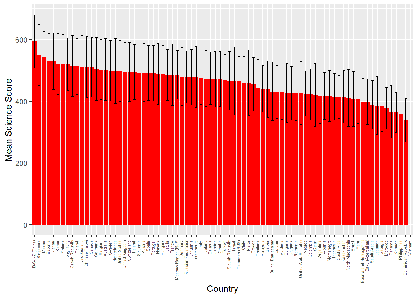
2.1 Task 1 Plot a graph of mean science scores by country
Imagine we wish to compare the mean scores of students on the science element of PISA by plotting a bar graph. First you need to use the sumarise function to calculate means by countries. Then use ggplot with geom_col to create the graph. Extension task: add error bars for the standard deviations of science scores.
Show the code
# Task 1: Plot a graph of mean science scores by country# Create a variable avgscience - for every country (Group_by(CNT)) calculate the mean# science score (PV1SCIE) and ignore NA (na.rm=TRUE)avgscience <- PISA_2018 %>%group_by(CNT) %>%summarise(mean_sci =mean(PV1SCIE, na.rm =TRUE)) %>%# Arrange in descending order arrange(desc(mean_sci))# Plot the data in avgscience, x=CNT (reorder to ascending order), mean science score on the y# Change the fill colour to red, rotate the text, locate the text and reduce the font sizeggplot(data = avgscience, aes(x =reorder(CNT, - mean_sci), y = mean_sci)) +geom_col(fill ="red") +theme(axis.text.x =element_text(angle =90, hjust =0.95, vjust =0.2, size =5))+labs(x ="Country", y ="Mean Science Score")
Show the code
# Extension version: added summarise to find standard deviation avgscience <- PISA_2018 %>%group_by(CNT) %>%summarise(mean_sci =mean(PV1SCIE, na.rm =TRUE),sd_sci =sd(PV1SCIE, na.rm =TRUE)) %>%arrange(desc(mean_sci))# Extension version: geom_errorbar added with aes y=mean_sci (the centre of the bar) and then the maximum and minimum set to the mean plus or minus the standard deviation (ymin=mean_sci-sd_sci, ymax=mean_sci+sd_sci) ggplot(data = avgscience, aes(x =reorder(CNT, -mean_sci), y = mean_sci)) +geom_col(fill ="red") +theme(axis.text.x =element_text(angle =90, hjust =0.95, vjust =0.2, size =5))+labs(x="Country", y ="Mean Science Score")+geom_errorbar(aes(y = mean_sci, ymin = mean_sci-sd_sci, ymax = mean_sci+sd_sci), width =0.5, colour='black', size =0.5)
2.2 Task 2 Are there differences in science scores by gender for the total data set?
Consider the kinds of variables that represent the science score. What is an appropriate test to determine differences in the means between the two groups? Create two vectors, for boys and girls, that you can feed into the t.test function.
Show the code
# Task 2: Are there differences in Science scores by gender for the total data set? (No)# A comparision of means of two continuous variables, use a t-test.# Choose the gender (ST004D01T) and science score columns (PV1SCIE) from 2018 data, filter for males # Put that data into MaleSciMaleSci <- PISA_2018 %>%select(ST004D01T, PV1SCIE) %>%filter(ST004D01T =="Male")# Choose the gender (ST004D01T) and science score columns (PV1SCIE) from 2018 data, filter for females # Put that data into FemaleSciFemaleSci <- PISA_2018 %>%select(CNT, ST004D01T, PV1SCIE) %>%filter(ST004D01T =="Female")#Do a t-test comparing MaleSci and FemaleScit.test(MaleSci$PV1SCIE, FemaleSci$PV1SCIE)
    Welch Two Sample t-test

data:  MaleSci$PV1SCIE and FemaleSci$PV1SCIE
t = -16.184, df = 604181, p-value < 2.2e-16
alternative hypothesis: true difference in means is not equal to 0
95 percent confidence interval:
 -4.781097 -3.748183
sample estimates:
mean of x mean of y
 458.5701  462.8347
2.3 Task 3 Are there differences in science scores by gender for UK students?
As above, but include a filter by country.
Show the code
# Task 3: Are there differences in Science scores by gender for UK students? (No)# A comparision of means of two continuous variables, use a t-test.# Choose the country (CNT), gender (ST004D01T) and science score columns (PV1SCIE) from 2018 data, filter for males and the UK# Put that data into UKMaleSciUKMaleSci <- PISA_2018 %>%select(CNT, ST004D01T, PV1SCIE) %>%filter(ST004D01T =="Male") %>%filter(CNT =="United Kingdom")# Choose the country (CNT), gender (ST004D01T) and science score columns (PV1SCIE) from 2018 data, filter for females and the UK# Put that data into UKFemaleSciUKFemaleSci <- PISA_2018 %>%select(CNT, ST004D01T, PV1SCIE) %>%filter(ST004D01T =="Female") %>%filter(CNT =="United Kingdom")# Do a t-test comparing UKMaleSci and UKFemaleScit.test(UKMaleSci$PV1SCIE, UKFemaleSci$PV1SCIE)
    Welch Two Sample t-test

data:  UKMaleSci$PV1SCIE and UKFemaleSci$PV1SCIE
t = -1.5274, df = 13662, p-value = 0.1267
alternative hypothesis: true difference in means is not equal to 0
95 percent confidence interval:
 -5.6282103  0.6983756
sample estimates:
mean of x mean of y
 493.9977  496.4626
2.4 Task 4 For the whole data set, is there a correlation between students’ science score and reading scores?
Reflect on the appropriate test to show correlation between two scores. This test can be carried out quite simply using a couple of lines of code. Extensions: a) perform the same analysis, but consider the impact of gender; b) Find the correlations between reading and science core by country, and rank from most highly correlated to least.
Show the code
# Task 4: For the whole data set, is there a correlation between students’ science score reading score? (Yes, significant 0.77)# Do the regression test between science score (PV1SCIE) and reading score (PV1READ) on the PISA_2018 datalmSciRead <-lm(PV1SCIE ~ PV1READ, data = PISA_2018)summary(lmSciRead)
Call:
lm(formula = PV1SCIE ~ PV1READ, data = PISA_2018)

Residuals:
     Min       1Q   Median       3Q      Max
-269.417  -32.284   -0.294   32.091  266.034

Coefficients:
             Estimate Std. Error t value Pr(>|t|)
(Intercept) 7.904e+01  2.710e-01   291.7   <2e-16 ***
PV1READ     8.367e-01  5.781e-04  1447.5   <2e-16 ***
---
Signif. codes:  0 '***' 0.001 '**' 0.01 '*' 0.05 '.' 0.1 ' ' 1

Residual standard error: 48.65 on 606625 degrees of freedom
  (5377 observations deleted due to missingness)
Multiple R-squared:  0.7755,    Adjusted R-squared:  0.7755
F-statistic: 2.095e+06 on 1 and 606625 DF,  p-value: < 2.2e-16
Call:
lm(formula = PV1SCIE ~ PV1READ + ST004D01T, data = PISA_2018)

Residuals:
     Min       1Q   Median       3Q      Max
-260.116  -31.457   -0.122   31.380  274.778

Coefficients:
               Estimate Std. Error t value Pr(>|t|)
(Intercept)   6.256e+01  2.821e-01   221.7   <2e-16 ***
PV1READ       8.499e-01  5.702e-04  1490.5   <2e-16 ***
ST004D01TMale 2.084e+01  1.232e-01   169.2   <2e-16 ***
---
Signif. codes:  0 '***' 0.001 '**' 0.01 '*' 0.05 '.' 0.1 ' ' 1

Residual standard error: 47.54 on 606622 degrees of freedom
  (5379 observations deleted due to missingness)
Multiple R-squared:  0.7856,    Adjusted R-squared:  0.7856
F-statistic: 1.111e+06 on 2 and 606622 DF,  p-value: < 2.2e-16
Show the code
# Extentions 2: Rank by correlation CNTPISA<-PISA_2018%>%select(CNT, PV1SCIE, PV1READ)%>%group_by(CNT)%>%summarise(MeanSci=mean(PV1SCIE),MeanRead=mean(PV1READ),Cor=cor(PV1SCIE,PV1READ)) %>%arrange(desc(Cor))
2.5 Task 5 Plot a representation of UK students’ science score against reading score, with a linear best fit line.
It will help here to create a data.frame that contains a filtered version of the whole dataset you can pass to ggplot.
Show the code
# Task 5: Plot a representation of UK students’ science score against reading score.# Choose the three variables of interest, science score (PV1SCIE), reading score (PV1READ) and country (CNT)# and filter for the UK. Put the values into regplotdataregplotdata<- PISA_2018 %>%select(PV1SCIE, PV1READ, CNT) %>%filter(CNT =="United Kingdom")# Plot the data in regplotdata, set the science score on the x-xis and reading on y-axis, set the size, colour and alpha (transparency)# of points and add a linear ('lm') black lineggplot(data = regplotdata, aes(x = PV1SCIE, y = PV1READ)) +geom_point(size=0.5, colour="red", alpha=0.3) +geom_smooth(method ="lm", colour="black")+labs(x ="Science Score", y ="Reading score")
2.6 Task 6 Do girls and boys in the UK engage in different levels of environmental activism?
The PISA 2018 data set includes the variable ST222Q09HA (I participate in activities in favour of environmental protection). Determine if the data for girls and boys are homogenous (i.e. if the null hypothesis that girls and boys engage in the same levels of activism is true).
Show the code
# Task 6: Is there a relationship between UK boys' and girls' levels of enviromnental activism.chi_data <- PISA_2018 %>%select(CNT, ST004D01T, ST222Q09HA) %>%filter(CNT =="United Kingdom") %>%na.omit()# We wish to compare two categorical variables, gender (Male/Female) and engagement in enviromental activism (Yes/No)# Create a frequency tableActivismtable <- chi_data %>%group_by(ST004D01T, ST222Q09HA)%>%count()# Pivot the table to create a contingency tableActivismtable <-pivot_wider(Activismtable, names_from = ST222Q09HA, values_from = n)# Drop the first column for passing to chisq.testActivismtable <-subset(Activismtable, select =c("Yes","No"))# Perform the chisq.test on the datachisq.test(Activismtable)
    Pearson's Chi-squared test with Yates' continuity correction

data:  Activismtable
X-squared = 0.07963, df = 1, p-value = 0.7778
Show the code
# p-value= 0.7778 - accept the null hypothesis - boys and girls have similar levels of activism
2.7 Task 7 Does participation in environmental activism explain variation in science score for UK students?
Arguments have been made the students who know more science, might engage in more environmental activism. Determine what percentage of variation in UK science scores is explained by a) the variable ST222Q09HA (I participate in activities in favour of environmental protection); b) ST222Q04HA (I sign environmental petitions online); and c) ST222Q03HA (I choose certain products for ethical or environmental reasons).
Show the code
# Task 7: How much variability in science score is explained by participation in activism?# Explanation of variation is performed by carrying out an anova testUK_data <- PISA_2018 %>%select(CNT, PV1SCIE, ST222Q09HA, ST222Q04HA, ST222Q03HA) %>%filter(CNT =="United Kingdom") %>%na.omit()# Perform the anova testresaov <-aov(data = UK_data, PV1SCIE ~ST222Q09HA + ST222Q04HA + ST222Q03HA)summary(resaov)
#> Significant differences exist for ST222Q09HA (I participate in activities in favour of environmental protection) (Pr(>F)=0.00827) but not ST222Q04HA (signing petitions) (p=0.18540) or choosing products for ethical/environmental reasons (p=0.45662)# Determine the % of variation explainedlibrary(lsr)eta <-etaSquared(resaov)eta <-100*etaeta